This document describes a series of tests which uses computer simulated data to evaluate the performance of the LINC-NIRVANA Data Reduction Software (LN DRS). Each test focuses on an instrument/observation specific aspect regarding the data which are later on available for the reconstruction task. In addition possible actions are described which assist in dealing with some raw data properties.

Each test section is split in a short description of the purpose of the test, a detailed specification of the setup, a list of the simulated input data, a presentation of the reconstruction results, and a short discussion of recommended actions (optional)

All test described in this document follow a common scheme which includes:

1. Purpose: Description of the purpose of a specific test. This can be mapped to a specific observation condition.
2. Simulation setup: Complete test setup specification including a link to the (online available) generated imput data for the data reduction pipeline.
3. Simulated raw images: The input data is presented.
4. Results: All reconstruction results are presented including images, profiles through the reconstructions, and error measurements..
5. Actions: This section contains a description of possible actions which give the user hints how to deal with the test specific conditions..

Since the LINC-NIRVANA Data Reduction Software implements an instrument specific pipeline, all test share a common setup (see table 1).

The raw data for all tests were generated with a set of C-programs and a Bash-script. This Bash-script additionally generates the parameter files which are later used by the LN DRS pipeline implemented in IDL. The principle steps for generating the input raw data files used by the pipeline are:

1. Generate the reference pupil, psf, sky background, target, and calibrator images. The reference images are based on an ideal 22.8m single dish telescope (no center hole!).
2. Generate for each position angle an atmospheric psf where the properties of the atmosphere (including strehl) are given by the test setup. In the simulation of the raw images, the fringes are always vertical and the object is rotated.
3. Generate a raw image of the target for each position angle:
   1. Convolve the target (no background) with the psf for that position angle.
   2. Rotate that image about the position angle to achieve vertical fringes.
   3. Add the flat sky background to that image.
   4. Apply poisson noise to the final image.
   At the end, all images are combined to an image cube.
4. Generate for each psf-star magnitude and position angle a raw psf-star image:
   • Convolve the psf-star (no background) with the psf for that position angle.
   • Rotate that image about the position angle to achieve vertical fringes.
   • Add the flat sky background to that image.
   • Apply poisson noise to the final image.
   At the end, all images for one brightness level are combined to an image cube.
5. For each brightness level a pipeline parameter file is generated.

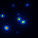
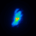
The basis of the simulations is an image of NGC4151 with an overlayed dust torus and a small star cluster. In figure 1 and figure 2 the images in J-Band and K-Band, convolved with the ideal 22.8m telescope psf are shown.

Figure 1: The reference images of NGC4151 at 10.1mag including sky background for the J-Band (left panel) and the K-Band (right panel).

Figure 2: The reference images of the star cluster including sky background for the J-Band (left panel) and the K-Band (right panel).

For some tests, the images for the target and calibrator are generated separately and sometimes later combined before the poisson noise is applied.

In the section discussing the reconstruction results, an error measurement is used which calculates the global difference between the ideal image and a reconstruction convolved with the ideal psf (both 23m psf). This measurement is described in the paper "K-H. Hofmann, T. Driebe, M. Heininger, D. Schertl and G. Weigelt, 2005, A&A, 444, 983-993".

A list of all test described in this document is given in table 3

• Scope
• Applicable documents
• External interfaces
• Acronyms and abbreviations
• Introduction
• Overview
• Dependency on the calibrator brightness
• Introduction
• Calibrator
• Raw Frames and Results for an AGN
• Raw Frames and Results for a Star Cluster
• Dependency on the strehl deviation
• Introduction
• Calibrator
• Raw Frames and Results for an AGN
• Raw Frames and Results for a Star Cluster
• Dependency on the FFTS performance
• Introduction
• Calibrator
• Raw Frames and Results for an AGN
• Raw Frames and Results for a Star Cluster
• Dependency on the OPD error
• Introduction
• Calibrator
• Dependency on the beam overlap
• Introduction
• Calibrator
• Raw Frames and Results for an AGN
• Raw Frames and Results for a Star Cluster
• Dependency on the target and calibrator spectrum
• Introduction
• Calibrator
• Raw Frames and Results for an AGN
• Raw Frames and Results for a Star Cluster
• Dependency on the atmospheric dispersion
• Introduction
• Calibrator
• Raw Frames and Results for an AGN
• Raw Frames and Results for a Star Cluster
• Dependency on the atmospheric dispersion and target and calibrator spectrum
• Introduction
• Calibrator
• Raw Frames and Results for an AGN
• Raw Frames and Results for a Star Cluster
• Dependency on the differences in the target and calibrator altitude
• Introduction
• Calibrator
• Raw Frames and Results for an AGN
• Raw Frames and Results for an Star Cluster
• Using an artificial psf for the deconvolution
• Introduction
• Calibrator
• Raw Frames and Results for an AGN
• Raw Frames and Results for a Star Cluster
• Using an artificial psf for the deconvolution
• Introduction
• Calibrator
• Raw Frames and Results for an AGN
• Raw Frames and Results for a star cluster

1. The reference images of NGC4151 at 10.1mag including sky background for the J-Band (left panel) and the K-Band (right panel).
2. The reference images of the star cluster including sky background for the J-Band (left panel) and the K-Band (right panel).
3. Central 128x128 pixels of the generated J-Band images of a calibrator at different magnitudes (from top left to bottomright: 14, 15, 16, 17, 18, 19, 20, 21, and 22mag).
4. Central 128x128 pixels of the generated K-Band images of a calibrator at different magnitudes (from top left to bottomright: 14, 15, 16, 17, 18, 19, 20, 21, and 22mag).
5. The simulated raw images for position angles of 108, 144, 180, 216, and 252 degree of NGC4151 at 10.1mag including sky background (top row J-Band, bottom row K-Band).
6. AGN: The J-Band reconstructions depending ion the calibrator brightness are shown in this figure. The top left image shown the reference image of NGC4151. The top right image shown the five coadded raw images. The second row show the reconstructions using the Richardson-Lucy algorithm. The calibrator brightness was 14 mag, 18 mag, and 22 mag (from left to right). In the third row, the Building-Block algorithm was used.
7. AGN: The K-Band reconstructions depending ion the calibrator brightness are shown in this figure. The top left image shown the reference image of NGC4151. The top right image shown the five coadded raw images. The second row show the reconstructions using the Richardson-Lucy algorithm. The calibrator brightness was 14 mag, 18 mag, and 22 mag (from left to right). In the third row, the Building-Block algorithm was used.
8. In this figure, the image errors depending on the calibrator brightness are shown.
9. Reconstruction error depending on the iteration number for the J-Band (left side) and the K-Band (right side). The reconstruction in the first row uses the Richardson-Lucy algorithm, in the second row, the Building-Block method was used.
10. Horizontal profile through the center of the reconstructed galaxy compared to the ideal image (J-Band). On the right side only the central part is shown. The reconstruction in the first row uses the Richardson-Lucy algorithm, in the second row, the Building-Block method was used.
11. Horizontal profile through the center of the reconstructed galaxy compared to the ideal image (K-Band). On the right side only the central part is shown. The reconstruction in the first row uses the Richardson-Lucy algorithm, in the second row, the Building-Block method was used.
12. The simulated raw images for position angles of 108, 144, 180, 216, and 252 degree of a star cluster including sky background (top row J-Band, bottom row K-Band).
13. Star cluster: The J-Band reconstructions depending ion the calibrator brightness are shown in this figure. The top left image shown the reference image of the star cluster. The top right image shown the five coadded raw images. The second row show the reconstructions using the Richardson-Lucy algorithm. The calibrator brightness was 14 mag, 18 mag, and 22 mag (from left to right). In the third row, the Building-Block algorithm was used.
14. Star cluster: The K-Band reconstructions depending ion the calibrator brightness are shown in this figure. The top left image shown the reference image of the star cluster. The top right image shown the five coadded raw images. The second row show the reconstructions using the Richardson-Lucy algorithm. The calibrator brightness was 14 mag, 18 mag, and 22 mag (from left to right). In the third row, the Building-Block algorithm was used.
15. In this figure, the image errors depending on the calibrator brightness are shown.
16. Photometric errors depending on the calibrator bightness in the J-Band (left side) and K-Band (right side). The reconstruction in the first row uses the Richardson-Lucy algorithm, in the second row, the Building-Block method was used.
17. Reconstruction error depending on the iteration number for the J-Band (left side) and the K-Band (right side). The reconstruction in the first row uses the Richardson-Lucy algorithm, in the second row, the Building-Block method was used.
18. Image and photometric errors depending on the iteration number in the J-Band (left side) and K-Band (right side). The calibrator brightness is 14 mag. The reconstruction in the first row uses the Richardson-Lucy algorithm, in the second row, the Building-Block method was used.
19. Image and photometric errors depending on the iteration number in the J-Band (left side) and K-Band (right side). The calibrator brightness is 18 mag. The reconstruction in the first row uses the Richardson-Lucy algorithm, in the second row, the Building-Block method was used.
20. Image and photometric errors depending on the iteration number in the J-Band (left side) and K-Band (right side). The calibrator brightness is 22 mag. The reconstruction in the first row uses the Richardson-Lucy algorithm, in the second row, the Building-Block method was used.
21. Central 128x128 pixels of the generated J-Band images of a calibrator at 14 mag and with different strehl (from top left to bottom right: 0.20, 0.25, 0.37, 0.29, 0.30, 0.31, 0.33, 0.35, and 0.40).
22. Central 128x128 pixels of the generated K-Band images of a calibrator at 14 mag and with different strehl (from top left to bottom right: 0.20, 0.25, 0.37, 0.29, 0.30, 0.31, 0.33, 0.35, and 0.40).
23. The simulated raw images for position angles of 108, 144, 180, 216, and 252 degree of a AGN including sky background (top row J-Band, bottom row K-Band).
24. AGN: The J-Band reconstructions depending on the calibrator strehl are shown in this figure. The top left image shown the reference image of NGC4151. The top right image shown the five coadded raw images. The second row show the reconstructions using the Richardson-Lucy algorithm. The calibrator strehl was 0.20, 0.30 (same as for the target), 0.40, and 1.0 (from left to right). In the third row, the Building-Block algorithm was used.
25. AGN: The K-Band reconstructions depending on the calibrator strehl are shown in this figure. The top left image shown the reference image of NGC4151. The top right image shown the five coadded raw images. The second row show the reconstructions using the Richardson-Lucy algorithm. The calibrator strehl was 0.20, 0.30 (same as for the target), 0.40, and 1.0 (from left to right). In the third row, the Building-Block algorithm was used.
26. In this figure, the image errors depending on the calibrator strehl ratio are shown.
27. Reconstruction error depending on the iteration number for the J-Band (left side) and K-Band (right side). In the first row, Richardson-Lucy was used for the reconstruction. In the second row, the Building-Block method was used.
28. Horizontal profile through the center of the reconstructed galaxy compared to the ideal image (J-Band). On the right side only the central part is shown. In the first row, Richardson-Lucy was used for the reconstruction. In the second row, the Building-Block method was used.
29. Horizontal profile through the center of the reconstructed galaxy compared to the ideal image (K-Band). On the right side only the central part is shown. In the first row, Richardson-Lucy was used for the reconstruction. In the second row, the Building-Block method was used.
30. The simulated raw images for position angles of 108, 144, 180, 216, and 252 degree of a star cluster including sky background (top row J-Band, bottom row K-Band).
31. Star cluster: The J-Band reconstructions depending on the calibrator strehl are shown in this figure. The top left image shown the reference image of the star cluster. The top right image shown the five coadded raw images. The second row show the reconstructions using the Richardson-Lucy algorithm. The calibrator strehl was 0.20, 0.30 (same as for the target), 0.40, and 1.0 (from left to right). In the third row, the Building-Block algorithm was used.
32. Star cluster: The K-Band reconstructions depending on the calibrator strehl are shown in this figure. The top left image shown the reference image of the star cluster. The top right image shown the five coadded raw images. The second row show the reconstructions using the Richardson-Lucy algorithm. The calibrator strehl was 0.20, 0.30 (same as for the target), 0.40, and 1.0 (from left to right). In the third row, the Building-Block algorithm was used.
33. In this figure, the image errors depending on the calibrator strehl ratio are shown.
34. Photometric errors depending on the calibrator strehl ratio in the J-Band (left side) and K-Band (right side). The reconstruction in the first row uses the Richardson-Lucy algorithm, in the second row, the Building-Block method was used.
35. Reconstruction error depending on the iteration number for the J-Band (left side) and K-Band (right side). In the first row, Richardson-Lucy was used for the reconstruction. In the second row, the Building-Block method was used.
36. Image and photometric errors depending on the iteration number in the J-Band (left side) and K-Band (right side). The calibrator has a strehl of 0.20. In the first row, Richardson-Lucy was used for the reconstruction. In the second row, the Building-Block method was used.
37. Image and photometric errors depending on the iteration number in the J-Band (left side) and K-Band (right side). The calibrator has a strehl of 0.30. In the first row, Richardson-Lucy was used for the reconstruction. In the second row, the Building-Block method was used.
38. Image and photometric errors depending on the iteration number in the J-Band (left side) and K-Band (right side). The calibrator has a strehl of 0.40. In the first row, Richardson-Lucy was used for the reconstruction. In the second row, the Building-Block method was used.
39. Image and photometric errors depending on the iteration number in the J-Band (left side) and K-Band (right side). The calibrator has a strehl of 1.00. In the first row, Richardson-Lucy was used for the reconstruction. In the second row, the Building-Block method was used.
40. Central 128x128 pixels of the generated J-Band (top row) and K-Band (bottpon row) images of a calibrator with phase errors of (from top left to bottom right) 0.0, 0.1, 0.2, and 0.5 lambda.
41. The simulated J-Band (top row) and K-Band (bottom row) raw images for a position angle of 108 degree of NGC4151 at 10.1 mag including sky background with a phase error of 0.0, 0.1, 0.2, and 0.5 lambda (from left to right).
42. The top row shows the coadded J-Band raw images. The second row show the reconstructions using the Richardson-Lucy algorithm. The phase error is 0.0, 0.1, 0.2, and 0.5 lambda (from left to right). In the third row, the Building-Block algorithm was used
43. The top row shows the coadded K-Band raw images. The second row show the reconstructions using the Richardson-Lucy algorithm. The phase error is 0.0, 0.1, 0.2, and 0.5 lambda (from left to right). In the third row, the Building-Block algorithm was used.
44. In this figure, the image errors depending on the phase error jitter are shown.
45. Reconstruction error depending on the iteration number for the J-Band (left side) and K-Band (right side). For the reconstructions in the top row, Richardson-Lucy was used. In the second row, the Building-Block algorithm was used.
46. Horizontal profile through the center of the reconstructed galaxy compared to the ideal image (J-Band). On the right side only the central part is shown. For the reconstructions in the top row, Richardson-Lucy was used. In the second row, the Building-Block algorithm was used.
47. Horizontal profile through the center of the reconstructed galaxy compared to the ideal image (K-Band). On the right side only the central part is shown. For the reconstructions in the top row, Richardson-Lucy was used. In the second row, the Building-Block algorithm was used.
48. The simulated J-Band (top row) and K-Band (bottom row) raw images for a position angle of 108 degree of the star cluster at 10.1 mag including sky background with a phase error of 0.0, 0.1, 0.2, and 0.5 lambda (from left to right).
49. The top row shows the coadded J-Band raw images. The second row show the reconstructions using the Richardson-Lucy algorithm. The phase error is 0.0, 0.1, 0.2, and 0.5 lambda (from left to right). In the third row, the Building-Block algorithm was used
50. The top row shows the coadded K-Band raw images. The second row show the reconstructions using the Richardson-Lucy algorithm. The phase error is 0.0, 0.1, 0.2, and 0.5 lambda (from left to right). In the third row, the Building-Block algorithm was used
51. In this figure, the image errors depending on the phase error jitter are shown.
52. Photometric errors depending on the phase error jitter in the J-Band (left side) and K-Band (right side). The reconstruction in the first row uses the Richardson-Lucy algorithm, in the second row, the Building-Block method was used.
53. Reconstruction error depending on the iteration number for the J-Band (left side) and K-Band (right side). For the reconstructions in the top row, Richardson-Lucy was used. In the second row, the Building-Block algorithm was used.
54. Image and photometric errors depending on the iteration number in the J-Band (left side) and K-Band (right side). The phase error is 0.0. For the reconstructions in the top row, Richardson-Lucy was used. In the second row, the Building-Block algorithm was used.
55. Image and photometric errors depending on the iteration number in the J-Band (left side) and K-Band (right side). The phase error is 0.1. For the reconstructions in the top row, Richardson-Lucy was used. In the second row, the Building-Block algorithm was used.
56. Image and photometric errors depending on the iteration number in the J-Band (left side) and K-Band (right side). The phase error is 0.2. For the reconstructions in the top row, Richardson-Lucy was used. In the second row, the Building-Block algorithm was used.
57. Image and photometric errors depending on the iteration number in the J-Band (left side) and K-Band (right side). The phase error is 0.5. For the reconstructions in the top row, Richardson-Lucy was used. In the second row, the Building-Block algorithm was used.
58. Central 128x128 pixels of the generated J-Band images of a calibrator with phase error offsets of 0.0, 0.05, 0.1, 0.2, 0.3, 0.4, and 0.5 lambda (from top to bottom) and phase error offsets of 0.0, 0.05, 0.1, and 0.2 lambda (from left to right) .
59. Central 128x128 pixels of the generated K-Band images of a calibrator with phase error offsets of 0.0, 0.05, 0.1, 0.2, 0.3, 0.4, and 0.5 lambda (from top to bottom) and phase error offsets of 0.0, 0.05, 0.1, and 0.2 lambda (from left to right) .
60. Central 128x128 pixels of the generated J-Band (top row) and K-Band (bottom row) images of a calibrator with overlap errors of 0.0 (no jitter), 0.2 (jitter 0.1), 0.6 (jitter 0.1), and 1.0 (jitter 0.1).
61. Central 128x128 pixels of the generated J-Band (top row) and K-Band (bottom row) images of NGC4151 with overlap errors of 0.0 (no jitter), 0.2 (jitter 0.1), 0.6 (jitter 0.1), and 1.0 (jitter 0.1).
62. The top row shows the central part of the coadded J-Band images of NGC4151 with overlap errors of 0.0 (no jitter), 0.2 (jitter 0.1), 0.6 (jitter 0.1), and 1.0 (jitter 0.1). In the second row, the reconstructions using the Richardson-Lucy algorithm are shown and in the third row, the Building-Block method was used.
63. The top row shows the central part of the coadded K-Band images of NGC4151 with overlap errors of 0.0 (no jitter), 0.2 (jitter 0.1), 0.6 (jitter 0.1), and 1.0 (jitter 0.1). In the second row, the reconstructions using the Richardson-Lucy algorithm are shown and in the third row, the Building-Block method was used.
64. In this figure, the image errors depending on the beam overlap are shown. The left column shows the J-Band values and in the right column, the K-Band values are shown. In the first row, Richardson-Lucy was used for the reconstruction. In the second row, the Building-Block method was used.
65. Reconstruction error depending on the iteration number for the J-Band (left side) and K-Band (right side). In the first row, Richardson-Lucy was used for the reconstruction. In the second row, the Building-Block method was used.
66. Horizontal profile through the center of the reconstructed galaxy compared to the ideal image (J-Band). On the right side only the central part is shown. In the first row, Richardson-Lucy was used for the reconstruction. In the second row, the Building-Block method was used.
67. Horizontal profile through the center of the reconstructed galaxy compared to the ideal image (K-Band). On the right side only the central part is shown. In the first row, Richardson-Lucy was used for the reconstruction. In the second row, the Building-Block method was used.
68. Central 128x128 pixels of the generated J-Band (top row) and K-Band (bottom row) images of the star cluster with overlap errors of 0.0 (no jitter), 0.2 (jitter 0.1), 0.6 (jitter 0.1), and 1.0 (jitter 0.1).
69. The top row shows the central part of the coadded J-Band images of the star cluster with overlap errors of 0.0 (no jitter), 0.2 (jitter 0.1), 0.6 (jitter 0.1), and 1.0 (jitter 0.1). In the second row, the reconstructions using the Richardson-Lucy algorithm are shown and in the third row, the Building-Block method was used.
70. The top row shows the central part of the coadded K-Band images of the star cluster with overlap errors of 0.0 (no jitter), 0.2 (jitter 0.1), 0.6 (jitter 0.1), and 1.0 (jitter 0.1). In the second row, the reconstructions using the Richardson-Lucy algorithm are shown and in the third row, the Building-Block method was used.
71. In this figure, the image errors depending on the beam overlap are shown. The left column shows the J-Band values and in the right column, the K-Band values are shown. In the first row, Richardson-Lucy was used for the reconstruction. In the second row, the Building-Block method was used.
72. Reconstruction error depending on the iteration number for the J-Band (left side) and K-Band (right side). In the first row, Richardson-Lucy was used for the reconstruction. In the second row, the Building-Block method was used.
73. Image and photometric errors depending on the iteration number in the J-Band (left side) and K-Band (right side). The overlap error is 0.0, 0.0. In the first row, Richardson-Lucy was used for the reconstruction. In the second row, the Building-Block method was used.
74. Image and photometric errors depending on the iteration number in the J-Band (left side) and K-Band (right side). The overlap error is 0.2, 0.1. In the first row, Richardson-Lucy was used for the reconstruction. In the second row, the Building-Block method was used.
75. Image and photometric errors depending on the iteration number in the J-Band (left side) and K-Band (right side). The overlap error is 0.6, 0.1. In the first row, Richardson-Lucy was used for the reconstruction. In the second row, the Building-Block method was used.
76. Image and photometric errors depending on the iteration number in the J-Band (left side) and K-Band (right side). The overlap error is 1.0, 0.1. In the first row, Richardson-Lucy was used for the reconstruction. In the second row, the Building-Block method was used.
77. Central 128x128 pixels of the generated J-Band (top row) and K-Band (bottom row) images of a calibrator with constant spectrum (left column), 0.1 mag brighter in the red (middle column), and 0.2 mag brighter in the red (right column).
78. The simulated J-Band (top row) ad K-Band (bottom row) raw images for a position angle of 108 degree of NGC4151 at 10.1mag including sky background. In the left column, a constant spectrum was used, in the right panel, the target was 0.5 mag brighter in the red.
79. NGC4151: In the first row, the coadded raw J-Band images are shown. For the reconstructions in the second row, the Richardson-Lucy algorithm was used and for the third row the Building-Block method was used. the target in the first two columns shows a constant spectrum, whereas for the last two columns, the target is 0.5 mag brighter in the red. In the first and third column, the calibrator shows a constant spectrum and in the second and fourth column, the calibrator is 0.2 mag brighter in the red.
80. NGC4151: In the first row, the coadded raw K-Band images are shown. For the reconstructions in the second row, the Richardson-Lucy algorithm was used and for the third row the Building-Block method was used. the target in the first two columns shows a constant spectrum, whereas for the last two columns, the target is 0.5 mag brighter in the red. In the first and third column, the calibrator shows a constant spectrum and in the second and fourth column, the calibrator is 0.2 mag brighter in the red.
81. Reconstruction error depending on the iteration number for the J-Band (left side) and K-Band (right side). For the first row, the Richardson-Lucy algorithm was used for the reconstruction. In the second row, the Building-Block method was used.
82. Horizontal profile through the center of the reconstructed galaxy compared to the ideal image (J-Band). On the right side only the central part is shown. For the first row, the Richardson-Lucy algorithm was used for the reconstruction. In the second row, the Building-Block method was used.
83. Horizontal profile through the center of the reconstructed galaxy compared to the ideal image (K-Band). On the right side only the central part is shown. For the first row, the Richardson-Lucy algorithm was used for the reconstruction. In the second row, the Building-Block method was used.
84. The simulated J-Band (top row) ad K-Band (bottom row) raw images for a position angle of 108 degree of a starcluster at 10.1mag including sky background. In the left column, a constant spectrum was used, in the right panel, the target was 0.5 mag brighter in the red.
85. Star cluster: In the first row, the coadded raw J-Band images are shown. For the reconstructions in the second row, the Richardson-Lucy algorithm was used and for the third row the Building-Block method was used. the target in the first two columns shows a constant spectrum, whereas for the last two columns, the target is 0.5 mag brighter in the red. In the first and third column, the calibrator shows a constant spectrum and in the second and fourth column, the calibrator is 0.2 mag brighter in the red.
86. Star cluster: In the first row, the coadded raw K-Band images are shown. For the reconstructions in the second row, the Richardson-Lucy algorithm was used and for the third row the Building-Block method was used. the target in the first two columns shows a constant spectrum, whereas for the last two columns, the target is 0.5 mag brighter in the red. In the first and third column, the calibrator shows a constant spectrum and in the second and fourth column, the calibrator is 0.2 mag brighter in the red.
87. Reconstruction error depending on the iteration number for the J-Band (left side) and K-Band (right side). For the first row, the Richardson-Lucy algorithm was used for the reconstruction. In the second row, the Building-Block method was used.
88. Image and photometric errors depending on the iteration number in the J-Band (left side) and K-Band (right side). Target and calibrator have a constant spectrum. For the first row, the Richardson-Lucy algorithm was used for the reconstruction. In the second row, the Building-Block method was used.
89. Image and photometric errors depending on the iteration number in the J-Band (left side) and K-Band (right side). The Target has a constant spectrum and the calibrator is 0.2 mag brighter in the red. For the first row, the Richardson-Lucy algorithm was used for the reconstruction. In the second row, the Building-Block method was used.
90. Image and photometric errors depending on the iteration number in the J-Band (left side) and K-Band (right side). The target is 0.5 mag brighter in the red and the calibrator has a constant spectrum. For the first row, the Richardson-Lucy algorithm was used for the reconstruction. In the second row, the Building-Block method was used.
91. Image and photometric errors depending on the iteration number in the J-Band (left side) and K-Band (right side). The Target is 0.5 mag brighter in the red and the calibrator is 0.2 mag brighter in the red. For the first row, the Richardson-Lucy algorithm was used for the reconstruction. In the second row, the Building-Block method was used.
92. Central 128x128 pixels of the generated J-Band calibrator images at a declination of -30 degree (first column), -20 degree (second column), 0 degree (third column), and +20 degree (fourth column). The first row contains the calibrator images where the position angle is smaller than 180 degree and the altitude is 15.6 degree, 16.5 degree, 15.1 degree, and 55.7 degree. The second row contain the calibrator images at culmination (altitudes 27.3 degree, 37.3 degree, 57.3 degree, and 77.3 degree).
93. Central 128x128 pixels of the generated K-Band calibrator images at a declination of -30 degree (first column), -20 degree (second column), 0 degree (third column), and +20 degree (fourth column). The first row contains the calibrator images where the position angle is smaller than 180 degree and the altitude is 15.6 degree, 16.5 degree, 15.1 degree, and 55.7 degree. The second row contain the calibrator images at culmination (altitudes 27.3 degree, 37.3 degree, 57.3 degree, and 77.3 degree).
94. Central 128x128 pixels of the generated J-Band NGC4151 images at a declination of -30 degree (first column), -20 degree (second column), 0 degree (third column), and +20 degree (fourth column). The first row contains the calibrator images where the position angle is smaller than 180 degree and the altitude is 15.6 degree, 16.5 degree, 15.1 degree, and 55.7 degree. The second row contain the AGN images at culmination (altitudes 27.3 degree, 37.3 degree, 57.3 degree, and 77.3 degree).
95. Central 128x128 pixels of the generated K-Band NGC4151 images at a declination of -30 degree (first column), -20 degree (second column), 0 degree (third column), and +20 degree (fourth column). The first row contains the calibrator images where the position angle is smaller than 180 degree and the altitude is 15.6 degree, 16.5 degree, 15.1 degree, and 55.7 degree. The second row contain the AGN images at culmination (altitudes 27.3 degree, 37.3 degree, 57.3 degree, and 77.3 degree).
96. Central 128x128 pixels of the coadded and reconstructed J-Band NGC4151 images at a declination of -30 degree (first column), -20 degree (second column), 0 degree (third column), and +20 degree (fourth column). The first row contains the coadded raw target images. The second row contain the reconstructions created with the Richardson-Lucy algorithm. For the third row, the Building-Block method was used.
97. Central 128x128 pixels of the coadded and reconstructed K-Band NGC4151 images at a declination of -30 degree (first column), -20 degree (second column), 0 degree (third column), and +20 degree (fourth column). The first row contains the coadded raw target images. The second row contain the reconstructions created with the Richardson-Lucy algorithm. For the third row, the Building-Block method was used.
98. In this figure, the image errors depending on the atmospheric dispersion are shown. The left column shows the J-Band values and in the right column, the K-Band values are shown. In the first row, Richardson-Lucy was used for the reconstruction. In the second row, the Building-Block method was used.
99. Reconstruction error depending on the iteration number for the J-Band (left side) and K-Band (right side). The first row contain the reconstructions created with the Richardson-Lucy algorithm. For the second row, the Building-Block method was used.
100. Horizontal profile through the center of the reconstructed galaxy compared to the ideal image (J-Band). On the right side only the central part is shown. The first row contain the reconstructions created with the Richardson-Lucy algorithm. For the second row, the Building-Block method was used.
101. Horizontal profile through the center of the reconstructed galaxy compared to the ideal image (K-Band). On the right side only the central part is shown. The first row contain the reconstructions created with the Richardson-Lucy algorithm. For the second row, the Building-Block method was used.
102. Central 128x128 pixels of the generated J-Band star cluster images at a declination of -30 degree (first column), -20 degree (second column), 0 degree (third column), and +20 degree (fourth column). The first row contains the calibrator images where the position angle is smaller than 180 degree and the altitude is 15.6 degree, 16.5 degree, 15.1 degree, and 55.7 degree. The second row contain the star cluster images at culmination (altitudes 27.3 degree, 37.3 degree, 57.3 degree, and 77.3 degree).
103. Central 128x128 pixels of the generated K-Band star cluster images at a declination of -30 degree (first column), -20 degree (second column), 0 degree (third column), and +20 degree (fourth column). The first row contains the calibrator images where the position angle is smaller than 180 degree and the altitude is 15.6 degree, 16.5 degree, 15.1 degree, and 55.7 degree. The second row contain the star cluster images at culmination (altitudes 27.3 degree, 37.3 degree, 57.3 degree, and 77.3 degree).
104. Central 128x128 pixels of the coadded and reconstructed J-Band star cluster images at a declination of -30 degree (first column), -20 degree (second column), 0 degree (third column), and +20 degree (fourth column). The first row contains the coadded raw target images. The second row contain the reconstructions created with the Richardson-Lucy algorithm. For the third row, the Building-Block method was used.
105. Central 128x128 pixels of the coadded and reconstructed K-Band star cluster images at a declination of -30 degree (first column), -20 degree (second column), 0 degree (third column), and +20 degree (fourth column). The first row contains the coadded raw target images. The second row contain the reconstructions created with the Richardson-Lucy algorithm. For the third row, the Building-Block method was used.
106. Reconstruction error depending on the iteration number for the J-Band (left side) and K-Band (right side). The first row contain the reconstructions created with the Richardson-Lucy algorithm. For the second row, the Building-Block method was used.
107. Image and photometric errors depending on the iteration number in the J-Band (left side) and K-Band (right side). The declination is -30 degree, the top row shows the results using the Richardson-Lucy algorithm, in the bottom row the Building-Block method was used.
108. Image and photometric errors depending on the iteration number in the J-Band (left side) and K-Band (right side). The declination is -20 degree, the top row shows the results using the Richardson-Lucy algorithm, in the bottom row the Building-Block method was used.
109. Image and photometric errors depending on the iteration number in the J-Band (left side) and K-Band (right side). The declination is 0 degree, the top row shows the results using the Richardson-Lucy algorithm, in the bottom row the Building-Block method was used.
110. Image and photometric errors depending on the iteration number in the J-Band (left side) and K-Band (right side). The declination is +20 degree, the top row shows the results using the Richardson-Lucy algorithm, in the bottom row the Building-Block method was used.
111. Central 128x128 pixels of the generated J-Band calibrator images at a declination of -30 degree (first column), -20 degree (second column), 0 degree (third column), and +20 degree (fourth column). The first row contains the calibrator images where the position angle is smaller than 180 degree and the altitude is 15.6 degree, 16.5 degree, 15.1 degree, and 55.7 degree. The second row contain the calibrator images at culmination (altitudes 27.3 degree, 37.3 degree, 57.3 degree, and 77.3 degree).
112. Central 128x128 pixels of the generated K-Band calibrator images at a declination of -30 degree (first column), -20 degree (second column), 0 degree (third column), and +20 degree (fourth column). The first row contains the calibrator images where the position angle is smaller than 180 degree and the altitude is 15.6 degree, 16.5 degree, 15.1 degree, and 55.7 degree. The second row contain the calibrator images at culmination (altitudes 27.3 degree, 37.3 degree, 57.3 degree, and 77.3 degree).
113. Central 128x128 pixels of the generated J-Band AGN images at a declination of -30 degree (first column), -20 degree (second column), 0 degree (third column), and +20 degree (fourth column). The first row contains the target images where the position angle is smaller than 180 degree and the altitude is 15.6 degree, 16.5 degree, 15.1 degree, and 55.7 degree. The second row contain the AGN images at culmination (altitudes 27.3 degree, 37.3 degree, 57.3 degree, and 77.3 degree).
114. Central 128x128 pixels of the generated K-Band AGN images at a declination of -30 degree (first column), -20 degree (second column), 0 degree (third column), and +20 degree (fourth column). The first row contains the target images where the position angle is smaller than 180 degree and the altitude is 15.6 degree, 16.5 degree, 15.1 degree, and 55.7 degree. The second row contain the AGN images at culmination (altitudes 27.3 degree, 37.3 degree, 57.3 degree, and 77.3 degree).
115. Central 128x128 pixels of the coadded and reconstructed J-Band NGC4151 images at a declination of -30 degree (first column), -20 degree (second column), 0 degree (third column), and +20 degree (fourth column). The first row contains the coadded raw target images. The second row contain the reconstructions created with the Richardson-Lucy algorithm. For the third row, the Building-Block method was used.
116. Central 128x128 pixels of the coadded and reconstructed K-Band NGC4151 images at a declination of -30 degree (first column), -20 degree (second column), 0 degree (third column), and +20 degree (fourth column). The first row contains the coadded raw target images. The second row contain the reconstructions created with the Richardson-Lucy algorithm. For the third row, the Building-Block method was used.
117. Reconstruction error depending on the iteration number for the J-Band (left side) and K-Band (right side). The first row contain the reconstructions created with the Richardson-Lucy algorithm. For the second row, the Building-Block method was used.
118. Horizontal profile through the center of the reconstructed galaxy compared to the ideal image (J-Band). On the left side only the central part is shown. The first row contain the reconstructions created with the Richardson-Lucy algorithm. For the second row, the Building-Block method was used.
119. Horizontal profile through the center of the reconstructed galaxy compared to the ideal image (K-Band). On the left side only the central part is shown. The first row contain the reconstructions created with the Richardson-Lucy algorithm. For the second row, the Building-Block method was used.
120. Central 128x128 pixels of the generated J-Band star cluster images at a declination of -30 degree (first column), -20 degree (second column), 0 degree (third column), and +20 degree (fourth column). The first row contains the calibrator images where the position angle is smaller than 180 degree and the altitude is 15.6 degree, 16.5 degree, 15.1 degree, and 55.7 degree. The second row contain the star cluster images at culmination (altitudes 27.3 degree, 37.3 degree, 57.3 degree, and 77.3 degree).
121. Central 128x128 pixels of the generated K-Band star cluster images at a declination of -30 degree (first column), -20 degree (second column), 0 degree (third column), and +20 degree (fourth column). The first row contains the calibrator images where the position angle is smaller than 180 degree and the altitude is 15.6 degree, 16.5 degree, 15.1 degree, and 55.7 degree. The second row contain the star cluster images at culmination (altitudes 27.3 degree, 37.3 degree, 57.3 degree, and 77.3 degree).
122. Central 128x128 pixels of the coadded and reconstructed J-Band star cluster images at a declination of -30 degree (first column), -20 degree (second column), 0 degree (third column), and +20 degree (fourth column). The first row contains the coadded raw target images. The second row contain the reconstructions created with the Richardson-Lucy algorithm. For the third row, the Building-Block method was used.
123. Central 128x128 pixels of the coadded and reconstructed K-Band star cluster images at a declination of -30 degree (first column), -20 degree (second column), 0 degree (third column), and +20 degree (fourth column). The first row contains the coadded raw target images. The second row contain the reconstructions created with the Richardson-Lucy algorithm. For the third row, the Building-Block method was used.
124. Reconstruction error depending on the iteration number for the J-Band (left side) and K-Band (right side). The first row contain the reconstructions created with the Richardson-Lucy algorithm. For the second row, the Building-Block method was used.
125. Image and photometric errors depending on the iteration number in the J-Band (left side) and K-Band (right side). The declination is -30 degree for the target and calibrator. The first row contain the reconstructions created with the Richardson-Lucy algorithm. For the second row, the Building-Block method was used.
126. Image and photometric errors depending on the iteration number in the J-Band (left side) and K-Band (right side). The declination is -20 degree for the target and calibrator. The first row contain the reconstructions created with the Richardson-Lucy algorithm. For the second row, the Building-Block method was used.
127. Image and photometric errors depending on the iteration number in the J-Band (left side) and K-Band (right side). The declination is 0 degree for the target and calibrator. The first row contain the reconstructions created with the Richardson-Lucy algorithm. For the second row, the Building-Block method was used.
128. Image and photometric errors depending on the iteration number in the J-Band (left side) and K-Band (right side). The declination is +20 degree for the target and calibrator. The first row contain the reconstructions created with the Richardson-Lucy algorithm. For the second row, the Building-Block method was used.
129. Central 128x128 pixels of the generated J-Band calibrator images at a declination of -30 degree. Each column contains the calibrator images for a specific position angle (from left to right: 144, 180, and 216 degree). Each row contains the calibrator images with a specific altitude difference (from top to bottom: -5.0, -1.0, 0.0, +1.0, +5.0 degree).
130. Central 128x128 pixels of the generated K-Band calibrator images at a declination of -30 degree. Each column contains the calibrator images for a specific position angle (from left to right: 144, 180, and 216 degree). Each row contains the calibrator images with a specific altitude difference (from top to bottom: -5.0, -1.0, 0.0, +1.0, +5.0 degree).
131. Central 128x128 pixels of the generated J-Band (top row) and K-Band (bottom row) AGN images at a declination of -30 degree (first column), -20 degree (second column), 0 degree (third column), and +20 degree (fourth column).
132. Central 128x128 pixels of the reconstructed J-Band NGC4151 images at a declination of -30 degree (first column), -20 degree (second column), 0 degree (third column), and +20 degree (fourth column). The target to calibrator differences are -5.0 degree for the first row, -1.0 degree for the second row, no difference for the third row, +1.0 degree for the fourth row, and +5.0 degree for the fifth row.
133. Central 128x128 pixels of the reconstructed K-Band NGC4151 images at a declination of -30 degree (first column), -20 degree (second column), 0 degree (third column), and +20 degree (fourth column). The target to calibrator differences are -5.0 degree for the first row, -1.0 degree for the second row, no difference for the third row, +1.0 degree for the fourth row, and +5.0 degree for the fifth row.
134. Reconstruction error depending on the target declination and altitude difference for the J-Band (left side) and K-Band (right side).
135. Horizontal profile through the center of the reconstructed galaxy compared to the ideal image (J-Band). On the left side only the central part is shown.
136. Horizontal profile through the center of the reconstructed galaxy compared to the ideal image (K-Band). On the left side only the central part is shown.
137. Central 128x128 pixels of the generated J-Band (top row) and K-Band (bottom row) star cluster images at a declination of -30 degree (first column), -20 degree (second column), 0 degree (third column), and +20 degree (fourth column).
138. Central 128x128 pixels of the reconstructed J-Band star cluster images at a declination of -30 degree (first column), -20 degree (second column), 0 degree (third column), and +20 degree (fourth column). The target to calibrator differences are -5.0 degree for the first row, -1.0 degree for the second row, no difference for the third row, +1.0 degree for the fourth row, and +5.0 degree for the fifth row.
139. Central 128x128 pixels of the reconstructed K-Band star cluster images at a declination of -30 degree (first column), -20 degree (second column), 0 degree (third column), and +20 degree (fourth column). The target to calibrator differences are -5.0 degree for the first row, -1.0 degree for the second row, no difference for the third row, +1.0 degree for the fourth row, and +5.0 degree for the fifth row.
140. Reconstruction error depending on the target declination and altitude difference for the J-Band (left side) and K-Band (right side).
141. Central 128x128 pixels of the generated J-Band images of a calibrator at 14 mag and with different strehl (from top left to bottom right: 0.10, 0.20, 0.30, 0.40, 0.50, 0.60, 0.70, 0.80, and 0.90).
142. Central 128x128 pixels of the generated K-Band images of a calibrator at 14 mag and with different strehl (from top left to bottom right: 0.10, 0.20, 0.30, 0.40, 0.50, 0.60, 0.70, 0.80, and 0.90).
143. This plot shows a comparison of the simulated and fitted AO halo in the J-Band (left side) and K-Band (right side).
144. The simulated J-Band raw images for different Strehl (0.10 at top left, to 1.0 at bottom right) and the position angle o180 degree of a AGN including sky background.
145. The simulated K-Band raw images for different Strehl (0.10 at top left, to 1.0 at bottom right) and the position angle o180 degree of a AGN including sky background.
146. AGN: J-Band reconstruction of an AGN. In the left column, the coadded raw image is presented. In the middle column, a reconstruction with Richardson-Lucy and the extracted calibrator PSF is shown. In the right column, the reconstruction with Richardson-Lucy and an artificial PSF is shown. The Strehl for the target and calibrator was 0.1, 0.2, 0.3, 0.4 and 0.5 (from top left to bottom right).
147. AGN: J-Band reconstruction of an AGN. In the left column, the coadded raw image is presented. In the middle column, a reconstruction with Richardson-Lucy and the extracted calibrator PSF is shown. In the right column, the reconstruction with Richardson-Lucy and an artificial PSF is shown. The Strehl for the target and calibrator was 0.6, 0.7, 0.8, 0.9 and 1.0 (from top left to bottom right).
148. AGN: K-Band reconstruction of an AGN. In the left column, the coadded raw image is presented. In the middle column, a reconstruction with Richardson-Lucy and the extracted calibrator PSF is shown. In the right column, the reconstruction with Richardson-Lucy and an artificial PSF is shown. The Strehl for the target and calibrator was 0.1, 0.2, 0.3, 0.4 and 0.5 (from top left to bottom right).
149. AGN: K-Band reconstruction of an AGN. In the left column, the coadded raw image is presented. In the middle column, a reconstruction with Richardson-Lucy and the extracted calibrator PSF is shown. In the right column, the reconstruction with Richardson-Lucy and an artificial PSF is shown. The Strehl for the target and calibrator was 0.6, 0.7, 0.8, 0.9 and 1.0 (from top left to bottom right).
150. Reconstruction error depending on the strehl ratio (left side: J-Band, right side: K-Band).
151. J-Band: Horizontal profile through the center of the reconstructed galaxy compared to the ideal image (left side: use the extracted PSF, right side: use an artificial PSF). In the bottom row only the central part is shown.
152. K-Band: Horizontal profile through the center of the reconstructed galaxy compared to the ideal image (left side: use the extracted PSF, right side: use an artificial PSF). In the bottom row only the central part is shown.
153. The simulated J-Band raw images for different Strehl (0.10 at top left, to 1.0 at bottom right) and the position angle o180 degree of a star cluster including sky background.
154. The simulated K-Band raw images for different Strehl (0.10 at top left, to 1.0 at bottom right) and the position angle o180 degree of a star cluster including sky background.
155. Star cluster: J-Band reconstruction of a star cluster. In the left column, the coadded raw image is presented. In the middle column, a reconstruction with Richardson-Lucy and the extracted calibrator PSF is shown. In the right column, the reconstruction with Richardson-Lucy and an artificial PSF is shown. The Strehl for the target and calibrator was 0.1, 0.2, 0.3, 0.4 and 0.5 (from top left to bottom right).
156. Star cluster: J-Band reconstruction of a star cluster. In the left column, the coadded raw image is presented. In the middle column, a reconstruction with Richardson-Lucy and the extracted calibrator PSF is shown. In the right column, the reconstruction with Richardson-Lucy and an artificial PSF is shown. The Strehl for the target and calibrator was 0.6, 0.7, 0.8, 0.9 and 1.0 (from top left to bottom right).
157. Star cluster: K-Band reconstruction of a star cluster. In the left column, the coadded raw image is presented. In the middle column, a reconstruction with Richardson-Lucy and the extracted calibrator PSF is shown. In the right column, the reconstruction with Richardson-Lucy and an artificial PSF is shown. The Strehl for the target and calibrator was 0.1, 0.2, 0.3, 0.4 and 0.5 (from top left to bottom right).
158. Star cluster: K-Band reconstruction of a star cluster. In the left column, the coadded raw image is presented. In the middle column, a reconstruction with Richardson-Lucy and the extracted calibrator PSF is shown. In the right column, the reconstruction with Richardson-Lucy and an artificial PSF is shown. The Strehl for the target and calibrator was 0.6, 0.7, 0.8, 0.9 and 1.0 (from top left to bottom right).
159. Reconstruction error depending on the strehl ratio (left side: J-Band, right side: K-Band).
160. Central 128x128 pixels of the generated J-Band images of a calibrator at different strehl ratios (from left to right: 0.05, 0.1, 0.2, 0.3, and 0.4) and magnitudes (from top to bottom: 14, 16, 18, 20, and 22mag).
161. Central 128x128 pixels of the generated K-Band images of a calibrator at different strehl ratios (from left to right: 0.05, 0.1, 0.2, 0.3, and 0.4) and magnitudes (from top to bottom: 14, 16, 18, 20, and 22mag).
162. The simulated raw images for a position angle of 180 degree of NGC4151 at 10.1mag including sky background at different strehl ratios (from left to right: 0.05, 0.1, 0.2, 0.3, and 0.4). The top row shows the J-Band, the bottom row shows the K-Band images.
163. AGN: The J-Band reconstructions depending on the calibrator brightness (second row to last row: 14.0 mag, 16.0 mag, 18.0 mag, 20.0 mag, and 22.0 mag) for a strehl ratio of 0.05. In the top row, the first image shows the J-Band reference image of NGC4151, the second image shows the five coadded J-Band raw images. The first column shows the results using the extracted PSF and the Richardson-Lucy algorithm. The second column shows the results using the modelled PSF and the Richardson-Lucy algorithm. In the third column, the Building-Block-Method uses the extracted PSF and the fourth column, the modelled PSF was used by the Building-Block-Method.
164. AGN: The K-Band reconstructions depending on the calibrator brightness (second row to last row: 14.0 mag, 16.0 mag, 18.0 mag, 20.0 mag, and 22.0 mag) for a strehl ratio of 0.05. In the top row, the first image shows the K-Band reference image of NGC4151, the second image shows the five coadded K-Band raw images. The first column shows the results using the extracted PSF and the Richardson-Lucy algorithm. The second column shows the results using the modelled PSF and the Richardson-Lucy algorithm. In the third column, the Building-Block-Method uses the extracted PSF and the fourth column, the modelled PSF was used by the Building-Block-Method.
165. AGN: The J-Band reconstructions depending on the calibrator brightness (second row to last row: 14.0 mag, 16.0 mag, 18.0 mag, 20.0 mag, and 22.0 mag) for a strehl ratio of 0.10. In the top row, the first image shows the J-Band reference image of NGC4151, the second image shows the five coadded J-Band raw images. The first column shows the results using the extracted PSF and the Richardson-Lucy algorithm. The second column shows the results using the modelled PSF and the Richardson-Lucy algorithm. In the third column, the Building-Block-Method uses the extracted PSF and the fourth column, the modelled PSF was used by the Building-Block-Method.
166. AGN: The K-Band reconstructions depending on the calibrator brightness (second row to last row: 14.0 mag, 16.0 mag, 18.0 mag, 20.0 mag, and 22.0 mag) for a strehl ratio of 0.10. In the top row, the first image shows the K-Band reference image of NGC4151, the second image shows the five coadded K-Band raw images. The first column shows the results using the extracted PSF and the Richardson-Lucy algorithm. The second column shows the results using the modelled PSF and the Richardson-Lucy algorithm. In the third column, the Building-Block-Method uses the extracted PSF and the fourth column, the modelled PSF was used by the Building-Block-Method.
167. AGN: The J-Band reconstructions depending on the calibrator brightness (second row to last row: 14.0 mag, 16.0 mag, 18.0 mag, 20.0 mag, and 22.0 mag) for a strehl ratio of 0.20. In the top row, the first image shows the J-Band reference image of NGC4151, the second image shows the five coadded J-Band raw images. The first column shows the results using the extracted PSF and the Richardson-Lucy algorithm. The second column shows the results using the modelled PSF and the Richardson-Lucy algorithm. In the third column, the Building-Block-Method uses the extracted PSF and the fourth column, the modelled PSF was used by the Building-Block-Method.
168. AGN: The K-Band reconstructions depending on the calibrator brightness (second row to last row: 14.0 mag, 16.0 mag, 18.0 mag, 20.0 mag, and 22.0 mag) for a strehl ratio of 0.20. In the top row, the first image shows the K-Band reference image of NGC4151, the second image shows the five coadded K-Band raw images. The first column shows the results using the extracted PSF and the Richardson-Lucy algorithm. The second column shows the results using the modelled PSF and the Richardson-Lucy algorithm. In the third column, the Building-Block-Method uses the extracted PSF and the fourth column, the modelled PSF was used by the Building-Block-Method.
169. AGN: The J-Band reconstructions depending on the calibrator brightness (second row to last row: 14.0 mag, 16.0 mag, 18.0 mag, 20.0 mag, and 22.0 mag) for a strehl ratio of 0.30. In the top row, the first image shows the J-Band reference image of NGC4151, the second image shows the five coadded J-Band raw images. The first column shows the results using the extracted PSF and the Richardson-Lucy algorithm. The second column shows the results using the modelled PSF and the Richardson-Lucy algorithm. In the third column, the Building-Block-Method uses the extracted PSF and the fourth column, the modelled PSF was used by the Building-Block-Method.
170. AGN: The K-Band reconstructions depending on the calibrator brightness (second row to last row: 14.0 mag, 16.0 mag, 18.0 mag, 20.0 mag, and 22.0 mag) for a strehl ratio of 0.30. In the top row, the first image shows the K-Band reference image of NGC4151, the second image shows the five coadded K-Band raw images. The first column shows the results using the extracted PSF and the Richardson-Lucy algorithm. The second column shows the results using the modelled PSF and the Richardson-Lucy algorithm. In the third column, the Building-Block-Method uses the extracted PSF and the fourth column, the modelled PSF was used by the Building-Block-Method.
171. AGN: The J-Band reconstructions depending on the calibrator brightness (second row to last row: 14.0 mag, 16.0 mag, 18.0 mag, 20.0 mag, and 22.0 mag) for a strehl ratio of 0.40. In the top row, the first image shows the J-Band reference image of NGC4151, the second image shows the five coadded J-Band raw images. The first column shows the results using the extracted PSF and the Richardson-Lucy algorithm. The second column shows the results using the modelled PSF and the Richardson-Lucy algorithm. In the third column, the Building-Block-Method uses the extracted PSF and the fourth column, the modelled PSF was used by the Building-Block-Method.
172. AGN: The K-Band reconstructions depending on the calibrator brightness (second row to last row: 14.0 mag, 16.0 mag, 18.0 mag, 20.0 mag, and 22.0 mag) for a strehl ratio of 0.40. In the top row, the first image shows the K-Band reference image of NGC4151, the second image shows the five coadded K-Band raw images. The first column shows the results using the extracted PSF and the Richardson-Lucy algorithm. The second column shows the results using the modelled PSF and the Richardson-Lucy algorithm. In the third column, the Building-Block-Method uses the extracted PSF and the fourth column, the modelled PSF was used by the Building-Block-Method.
173. In this figure, the image errors depending on the calibrator brightness are shown. This are the results for a strehl ratio of 0.05. The left panel shows the results for the J-Band, in the right panel, the K-band is shown.
174. In this figure, the image errors depending on the calibrator brightness are shown. This are the results for a strehl ratio of 0.10. The left panel shows the results for the J-Band, in the right panel, the K-band is shown.
175. In this figure, the image errors depending on the calibrator brightness are shown. This are the results for a strehl ratio of 0.20. The left panel shows the results for the J-Band, in the right panel, the K-band is shown.
176. In this figure, the image errors depending on the calibrator brightness are shown. This are the results for a strehl ratio of 0.30. The left panel shows the results for the J-Band, in the right panel, the K-band is shown.
177. In this figure, the image errors depending on the calibrator brightness are shown. This are the results for a strehl ratio of 0.40. The left panel shows the results for the J-Band, in the right panel, the K-band is shown.
178. The simulated raw images for a position angle of 180 degree of a star cluster including sky background at different strehl ratios (from left to right: 0.05, 0.1, 0.2, 0.3, and 0.4). The top row shows the J-Band, the bottom row shows the K-Band images.
179. Star cluster: The J-Band reconstructions depending on the calibrator brightness (second row to last row: 14.0 mag, 16.0 mag, 18.0 mag, 20.0 mag, and 22.0 mag) for a strehl ratio of 0.05. In the top row, the first image shows the J-Band reference image of the star cluster, the second image shows the five coadded J-Band raw images. The first column shows the results using the extracted PSF and the Richardson-Lucy algorithm. The second column shows the results using the modelled PSF and the Richardson-Lucy algorithm. In the third column, the Building-Block-Method uses the extracted PSF and the fourth column, the modelled PSF was used by the Building-Block-Method.
180. Star cluster: The K-Band reconstructions depending on the calibrator brightness (second row to last row: 14.0 mag, 16.0 mag, 18.0 mag, 20.0 mag, and 22.0 mag) for a strehl ratio of 0.05. In the top row, the first image shows the K-Band reference image of the star cluster, the second image shows the five coadded K-Band raw images. The first column shows the results using the extracted PSF and the Richardson-Lucy algorithm. The second column shows the results using the modelled PSF and the Richardson-Lucy algorithm. In the third column, the Building-Block-Method uses the extracted PSF and the fourth column, the modelled PSF was used by the Building-Block-Method.
181. Star cluster: The J-Band reconstructions depending on the calibrator brightness (second row to last row: 14.0 mag, 16.0 mag, 18.0 mag, 20.0 mag, and 22.0 mag) for a strehl ratio of 0.10. In the top row, the first image shows the J-Band reference image of the star cluster, the second image shows the five coadded J-Band raw images. The first column shows the results using the extracted PSF and the Richardson-Lucy algorithm. The second column shows the results using the modelled PSF and the Richardson-Lucy algorithm. In the third column, the Building-Block-Method uses the extracted PSF and the fourth column, the modelled PSF was used by the Building-Block-Method.
182. Star cluster: The K-Band reconstructions depending on the calibrator brightness (second row to last row: 14.0 mag, 16.0 mag, 18.0 mag, 20.0 mag, and 22.0 mag) for a strehl ratio of 0.10. In the top row, the first image shows the K-Band reference image of the star cluster, the second image shows the five coadded K-Band raw images. The first column shows the results using the extracted PSF and the Richardson-Lucy algorithm. The second column shows the results using the modelled PSF and the Richardson-Lucy algorithm. In the third column, the Building-Block-Method uses the extracted PSF and the fourth column, the modelled PSF was used by the Building-Block-Method.
183. Star cluster: The J-Band reconstructions depending on the calibrator brightness (second row to last row: 14.0 mag, 16.0 mag, 18.0 mag, 20.0 mag, and 22.0 mag) for a strehl ratio of 0.20. In the top row, the first image shows the J-Band reference image of the star cluster, the second image shows the five coadded J-Band raw images. The first column shows the results using the extracted PSF and the Richardson-Lucy algorithm. The second column shows the results using the modelled PSF and the Richardson-Lucy algorithm. In the third column, the Building-Block-Method uses the extracted PSF and the fourth column, the modelled PSF was used by the Building-Block-Method.
184. Star cluster: The K-Band reconstructions depending on the calibrator brightness (second row to last row: 14.0 mag, 16.0 mag, 18.0 mag, 20.0 mag, and 22.0 mag) for a strehl ratio of 0.20. In the top row, the first image shows the K-Band reference image of the star cluster, the second image shows the five coadded K-Band raw images. The first column shows the results using the extracted PSF and the Richardson-Lucy algorithm. The second column shows the results using the modelled PSF and the Richardson-Lucy algorithm. In the third column, the Building-Block-Method uses the extracted PSF and the fourth column, the modelled PSF was used by the Building-Block-Method.
185. Star cluster: The J-Band reconstructions depending on the calibrator brightness (second row to last row: 14.0 mag, 16.0 mag, 18.0 mag, 20.0 mag, and 22.0 mag) for a strehl ratio of 0.30. In the top row, the first image shows the J-Band reference image of the star cluster, the second image shows the five coadded J-Band raw images. The first column shows the results using the extracted PSF and the Richardson-Lucy algorithm. The second column shows the results using the modelled PSF and the Richardson-Lucy algorithm. In the third column, the Building-Block-Method uses the extracted PSF and the fourth column, the modelled PSF was used by the Building-Block-Method.
186. Star cluster: The K-Band reconstructions depending on the calibrator brightness (second row to last row: 14.0 mag, 16.0 mag, 18.0 mag, 20.0 mag, and 22.0 mag) for a strehl ratio of 0.30. In the top row, the first image shows the K-Band reference image of the star cluster, the second image shows the five coadded K-Band raw images. The first column shows the results using the extracted PSF and the Richardson-Lucy algorithm. The second column shows the results using the modelled PSF and the Richardson-Lucy algorithm. In the third column, the Building-Block-Method uses the extracted PSF and the fourth column, the modelled PSF was used by the Building-Block-Method.
187. Star cluster: The J-Band reconstructions depending on the calibrator brightness (second row to last row: 14.0 mag, 16.0 mag, 18.0 mag, 20.0 mag, and 22.0 mag) for a strehl ratio of 0.40. In the top row, the first image shows the J-Band reference image of the star cluster, the second image shows the five coadded J-Band raw images. The first column shows the results using the extracted PSF and the Richardson-Lucy algorithm. The second column shows the results using the modelled PSF and the Richardson-Lucy algorithm. In the third column, the Building-Block-Method uses the extracted PSF and the fourth column, the modelled PSF was used by the Building-Block-Method.
188. Star cluster: The K-Band reconstructions depending on the calibrator brightness (second row to last row: 14.0 mag, 16.0 mag, 18.0 mag, 20.0 mag, and 22.0 mag) for a strehl ratio of 0.40. In the top row, the first image shows the K-Band reference image of the star cluster, the second image shows the five coadded K-Band raw images. The first column shows the results using the extracted PSF and the Richardson-Lucy algorithm. The second column shows the results using the modelled PSF and the Richardson-Lucy algorithm. In the third column, the Building-Block-Method uses the extracted PSF and the fourth column, the modelled PSF was used by the Building-Block-Method.
189. In this figure, the image errors depending on the calibrator brightness are shown. This are the results for a strehl ratio of 0.05. The left panel shows the results for the J-Band, in the right panel, the K-band is shown.
190. In this figure, the image errors depending on the calibrator brightness are shown. This are the results for a strehl ratio of 0.10. The left panel shows the results for the J-Band, in the right panel, the K-band is shown.
191. In this figure, the image errors depending on the calibrator brightness are shown. This are the results for a strehl ratio of 0.20. The left panel shows the results for the J-Band, in the right panel, the K-band is shown.
192. In this figure, the image errors depending on the calibrator brightness are shown. This are the results for a strehl ratio of 0.30. The left panel shows the results for the J-Band, in the right panel, the K-band is shown.
193. In this figure, the image errors depending on the calibrator brightness are shown. This are the results for a strehl ratio of 0.40. The left panel shows the results for the J-Band, in the right panel, the K-band is shown.

1. Applicable documents
2. External interfaces
3. Acronyms and abbreviations
4. Common test setup
5. Parameters for the star cluster. The coordinates are given relative to a 512x512 pixel image.
6. List of all test cases.
7. Setup for the simulation in J-Band and K-Band, .
8. Reconstruction errors for the AGN depending on the psf star brightness (J-Band).
9. Reconstruction errors for the AGN depending on the psf star brightness (K-Band).
10. Reconstruction errors for the star cluster depending on the psf star brightness (J-Band).
11. Reconstruction errors for the star cluster depending on the psf star brightness (K-Band).
12. Setup for the simulation in J-Band and K-Band, for the common test setup see .
13. AGN: Errors depending on the calibrator strehl (J-Band).
14. AGN: Errors depending on the calibrator strehl (K-Band).
15. Star cluster: Errors depending on the calibrator strehl (J-Band).
16. Star cluster: Errors depending on the calibrator strehl (K-Band).
17. Setup for the simulation in J-Band and K-Band, for the common test setup see .
18. AGN: Errors depending on the OPD error (J-Band).
19. AGN: Errors depending on the OPD error (K-Band).
20. Star cluster: Errors depending on the OPD error (J-Band).
21. Star cluster: Errors depending on the OPD error(K-Band).
22. Setup for the simulation in J-Band and K-Band, for the common test setup see .
23. Setup for the simulation in J-Band and K-Band, for the common test setup see .
24. AGN: Errors depending on the beam overlap error (J-Band).
25. AGN: Errors depending on the beam overlap error (K-Band).
26. Star cluster: Errors depending on the beam position error (J-Band).
27. Star cluster: Errors depending on the beam position error (K-Band).
28. Setup for the simulation in J-Band and K-Band, for the common test setup see .
29. AGN: Errors depending on the target and calibrator spectrum (J-Band).
30. AGN: Errors depending on the target and calibrator spectrum (K-Band).
31. Star cluster: Errors depending on the target and calibrator spectrum (J-Band).
32. Star cluster: Errors depending on the target and calibrator spectrum (K-Band).
33. Setup for the simulation in J-Band and K-Band, for the common test setup see .
34. Combinations of declination, culmination, smallest altitude, and achieved parallactic angles for target and calibrator.
35. AGN: Errors depending on the atmospheric dispersion (J-Band).
36. AGN: Errors depending on the atmospheric dispersion (K-Band).
37. Star cluster: Errors depending on the atmospheric dispersion (J-Band).
38. Star cluster: Errors depending on the atmospheric dispersion (K-Band).
39. Setup for the simulation in J-Band and K-Band, for the common test setup see .
40. Combinations of declination, culmination, smallest altitude, and achieved parallactic angles for target and calibrator.
41. NGC4151: Errors depending on the atmospheric dispersion (short side of the J-Band).
42. NGC4151: Errors depending on the atmospheric dispersion (K-Band).
43. Star cluster: Errors depending on the atmospheric dispersion (short side of the J-Band).
44. Star cluster: Errors depending on the atmospheric dispersion (K-Band).
45. Setup for the simulation in J-Band and K-Band, for the common test setup see .
46. Combinations of declination, culmination, smallest altitude, and achieved parallactic angles for target and calibrator.
47. NGC4151: Errors depending on the altitude difference between target and calibrator (short side of the J-Band).
48. NGC4151: Errors depending on the altitude difference between target and calibrator (K-Band).
49. Star cluster: Errors depending on the altitude difference between target and calibrator (short side of the J-Band).
50. Star cluster: Errors depending on the altitude difference between target and calibrator (K-Band).
51. Setup for the simulation in J-Band and K-Band, for the common test setup see .
52. AGN: Errors depending on the PSF creation method (J-Band).
53. AGN: Errors depending on the PSF creation method (K-Band).
54. Star cluster: Errors depending on the PSF creation method (J-Band).
55. Star cluster: Errors depending on the PSF creation method (K-Band).
56. Reconstruction errors for the AGN depending on the psf star brightness and strehl ratio (J-Band).
57. Reconstruction errors for the AGN depending on the psf star brightness and strehl ratio (K-Band).
58. Reconstruction errors for the star cluster depending on the psf star brightness and strehl ratio (J-Band).
59. Reconstruction errors for the star cluster depending on the psf star brightness and strehl ratio (K-Band).