In some observation conditions the psf of the target is not equal to the psf of the calibrator. Several reasons for the discrepancies do exist. For this test case different AO-performances for the target and calibrator are assumed which result in different strehl values. Unequal spectra of the target and the calibrator or other sources for discrepancies are not coverd by this test case.

The setup of the simulation is described in table 1. The input data for the test uses a raw target image with a strehl of 30 percent and the strehl of the psf-star covers a range from 20 percent up to 40 percent. In addition an artificial perfect psf (strehl 100 percent) is used for the reconstruction. In this experiment a bright psf star is chosen (14 mag), so that the reconstructions are not influenced by the photon noise of the calibrator.

The raw data were generated according to the common scheme described in section Overview. In addition the images for the target and psf-star are generated separately which means, that the psf-star image is not influenced by the target (no halo, etc.).

All simulated input data for the LN DRS pipeline are available as a tar-file (ex2_j_input.tar.gz (18MB) and ex2_k_input.tar.gz (21MB)). The corresponding results are also available as tar files (ex2_j_results.tar.gz (5.5MB) and ex2_k_results.tar.gz (5.7MB)).

The generated calibrator raw images are shown in section Calibrator. The raw images and deconvolution results are shown in section Raw Frames and Results for an AGN for the AGN and section Raw Frames and Results for a Star Cluster for the star cluster.

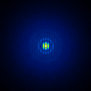
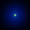
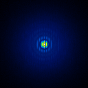
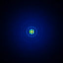
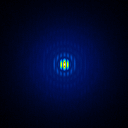
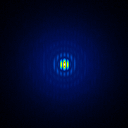
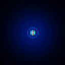
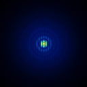
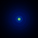
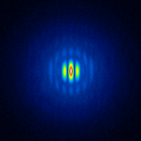
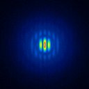
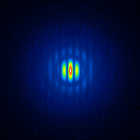
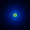
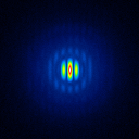
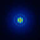
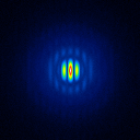
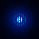
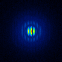
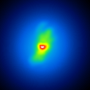
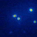
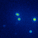
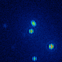
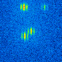
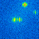
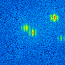
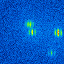
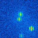
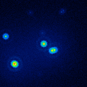
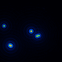
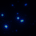
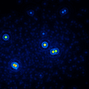
The simulated raw LBT interferograms used for the deconvolution are ideal images, they are not influenced by detector effects like different pixel gain or bad pixels. In figure 1 (J-Band) and figure 2 (K-Band) the calibrator for some strehl values are shown.

Figure 1: Central 128x128 pixels of the generated J-Band images of a calibrator at 14 mag and with different strehl (from top left to bottom right: 0.20, 0.25, 0.37, 0.29, 0.30, 0.31, 0.33, 0.35, and 0.40).

Figure 2: Central 128x128 pixels of the generated K-Band images of a calibrator at 14 mag and with different strehl (from top left to bottom right: 0.20, 0.25, 0.37, 0.29, 0.30, 0.31, 0.33, 0.35, and 0.40).

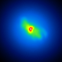
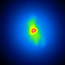
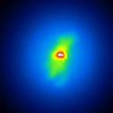
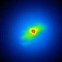
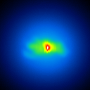
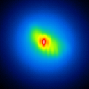
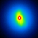
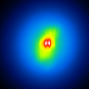
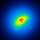
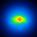
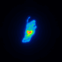
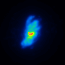
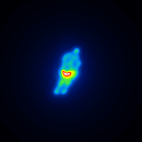
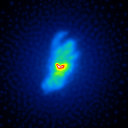
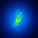
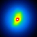
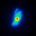
The basis of this simulation is an image of NGC4151 with an overlayed dust torus (see figure 1). The simulated raw images are shown in figure 3.

Figure 3: The simulated raw images for position angles of 108, 144, 180, 216, and 252 degree of a AGN including sky background (top row J-Band, bottom row K-Band).

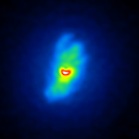
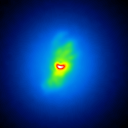
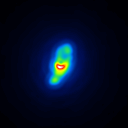
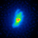
A comparison of the reconstructions depending on the calibrator strehl is presented in figure 4 (J-Band) and figure 5 (K-Band).

Figure 4: AGN: The J-Band reconstructions depending on the calibrator strehl are shown in this figure. The top left image shown the reference image of NGC4151. The top right image shown the five coadded raw images. The second row show the reconstructions using the Richardson-Lucy algorithm. The calibrator strehl was 0.20, 0.30 (same as for the target), 0.40, and 1.0 (from left to right). In the third row, the Building-Block algorithm was used.

Figure 5: AGN: The K-Band reconstructions depending on the calibrator strehl are shown in this figure. The top left image shown the reference image of NGC4151. The top right image shown the five coadded raw images. The second row show the reconstructions using the Richardson-Lucy algorithm. The calibrator strehl was 0.20, 0.30 (same as for the target), 0.40, and 1.0 (from left to right). In the third row, the Building-Block algorithm was used.

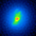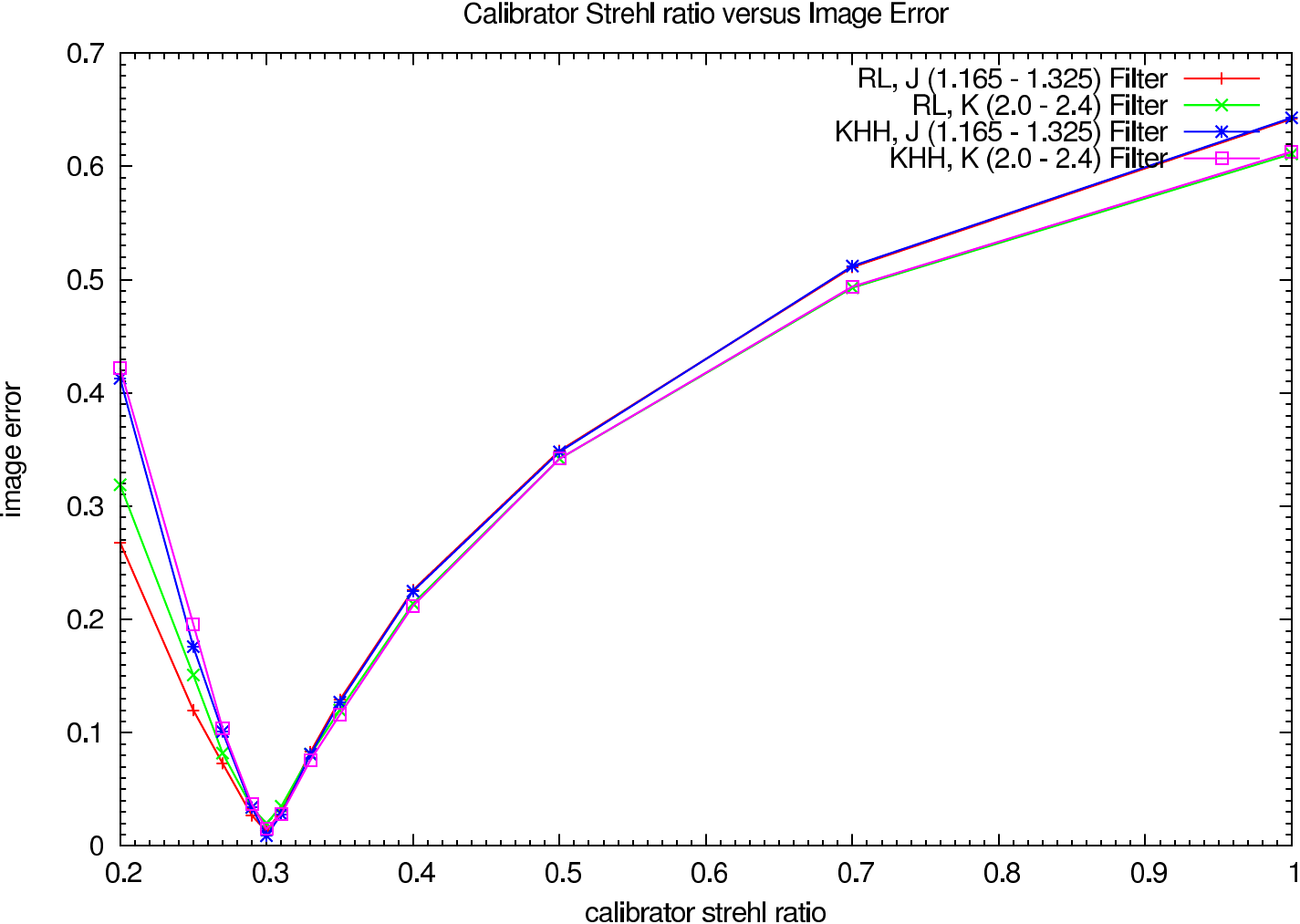
In table 2 (J-Band) and table 3 (K-Band) the errors for the star cluster depending on the calibrator strehl are presented. In figure 6 the image errors depending on the calibrator strehl ratio are shown.

Figure 6: In this figure, the image errors depending on the calibrator strehl ratio are shown.

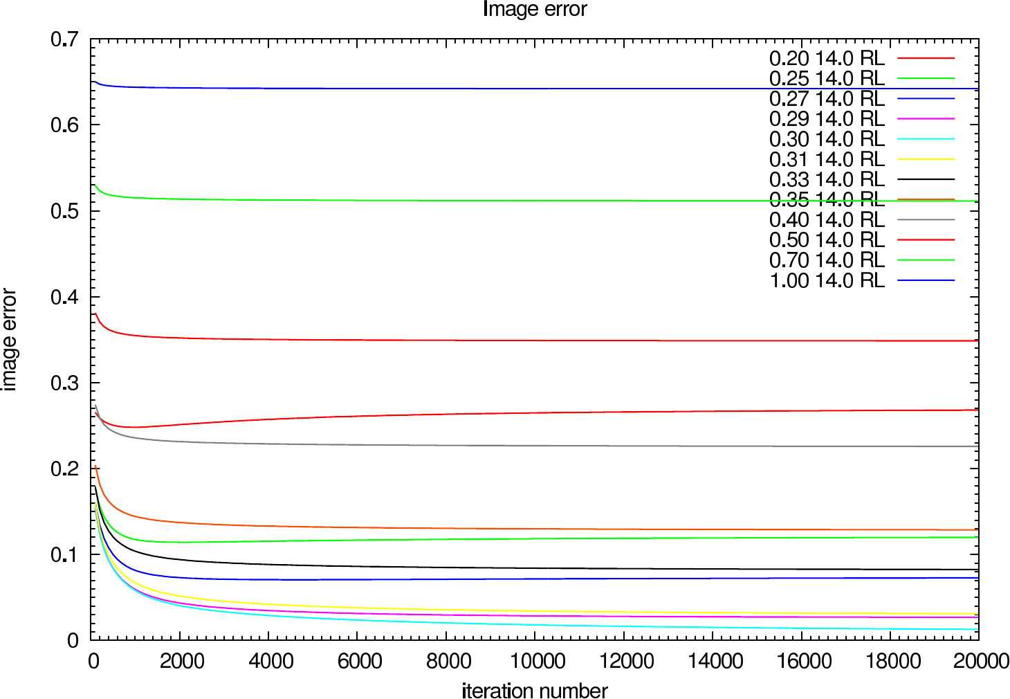
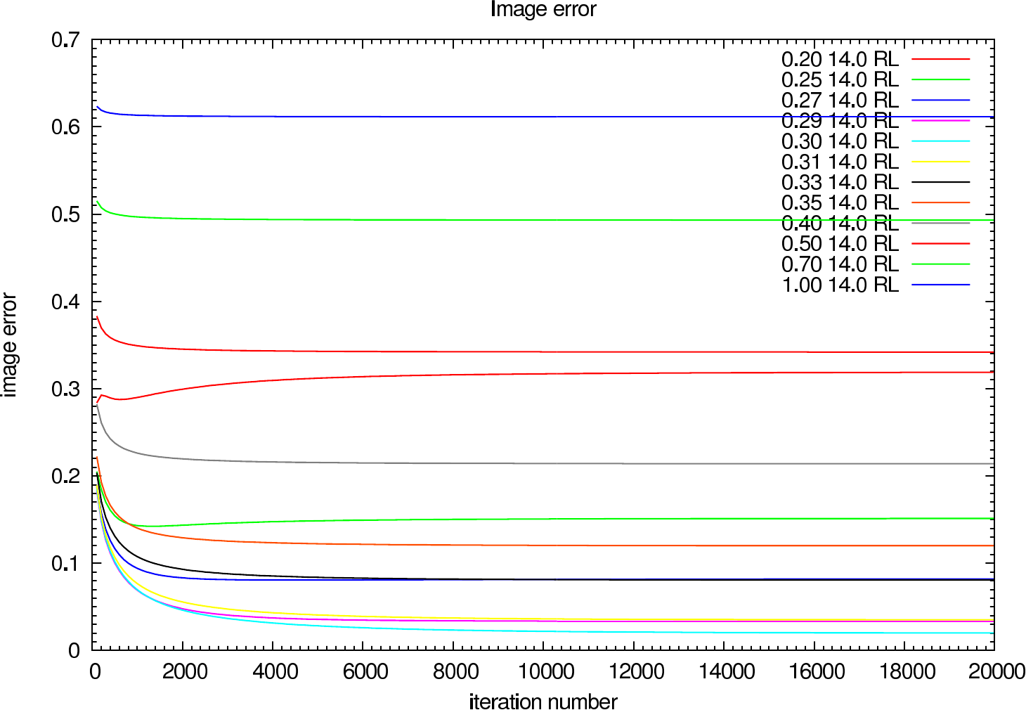
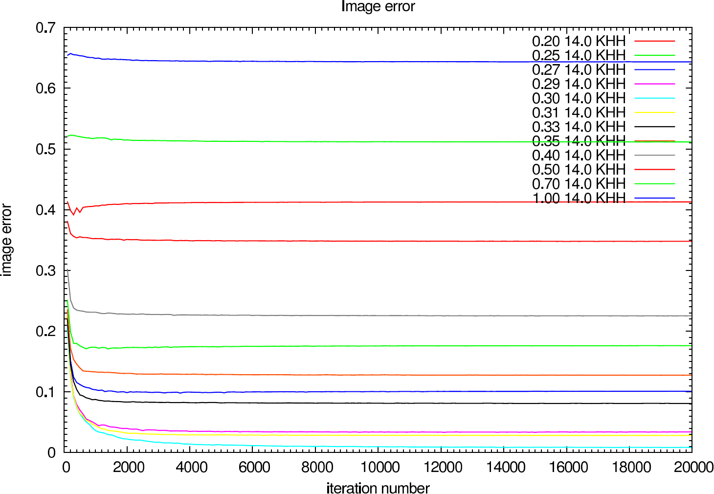
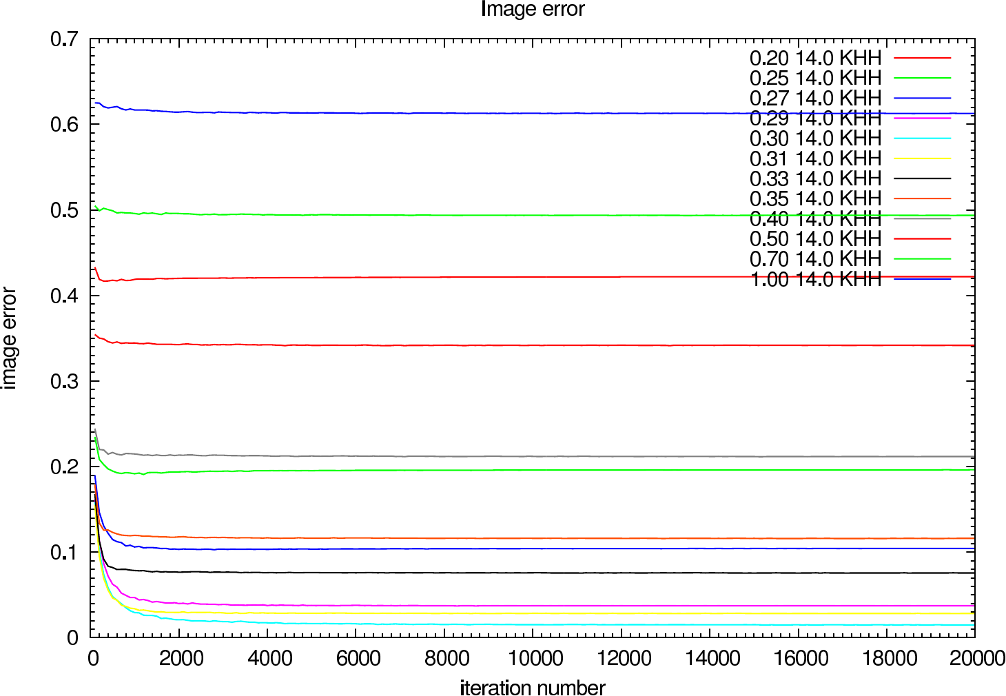
In figure 7 the image error describing the difference between the reconstruction and the reference image is shown for each iteration (in steps of 100 iterations). The effect of the calibrator strehl on the reconstruction error and the optimal iteration number is clearly visible.

Figure 7: Reconstruction error depending on the iteration number for the J-Band (left side) and K-Band (right side). In the first row, Richardson-Lucy was used for the reconstruction. In the second row, the Building-Block method was used.

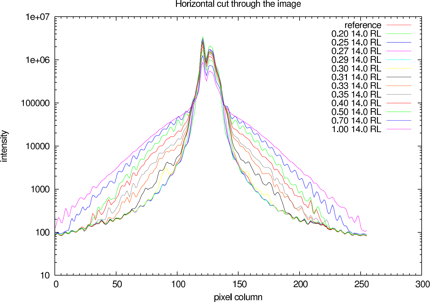
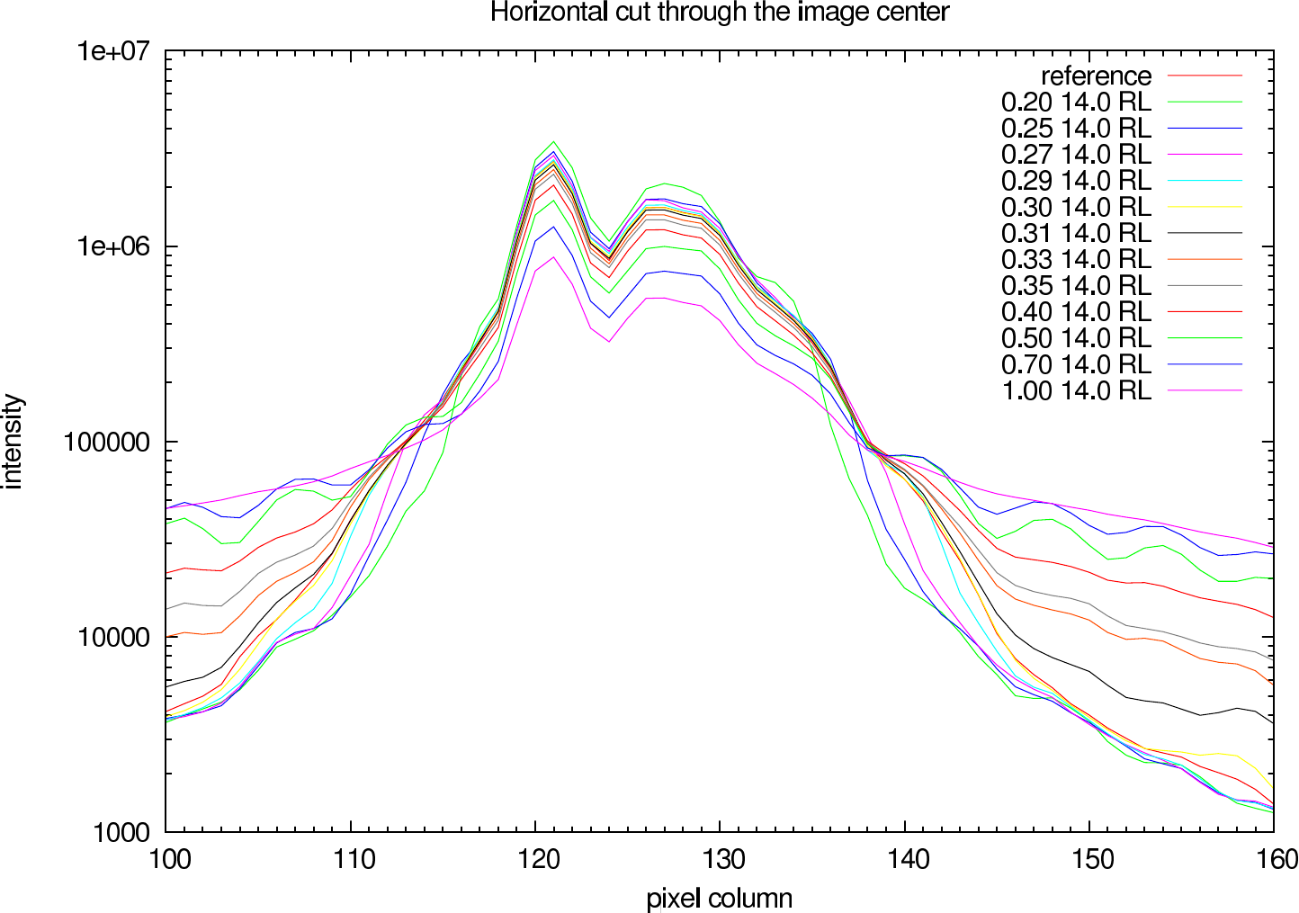
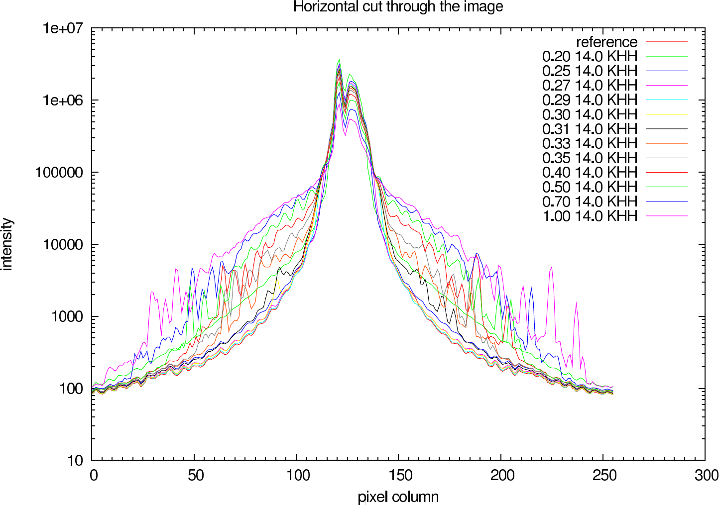
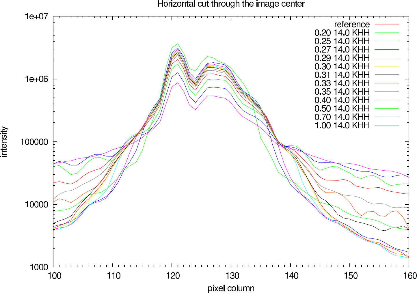
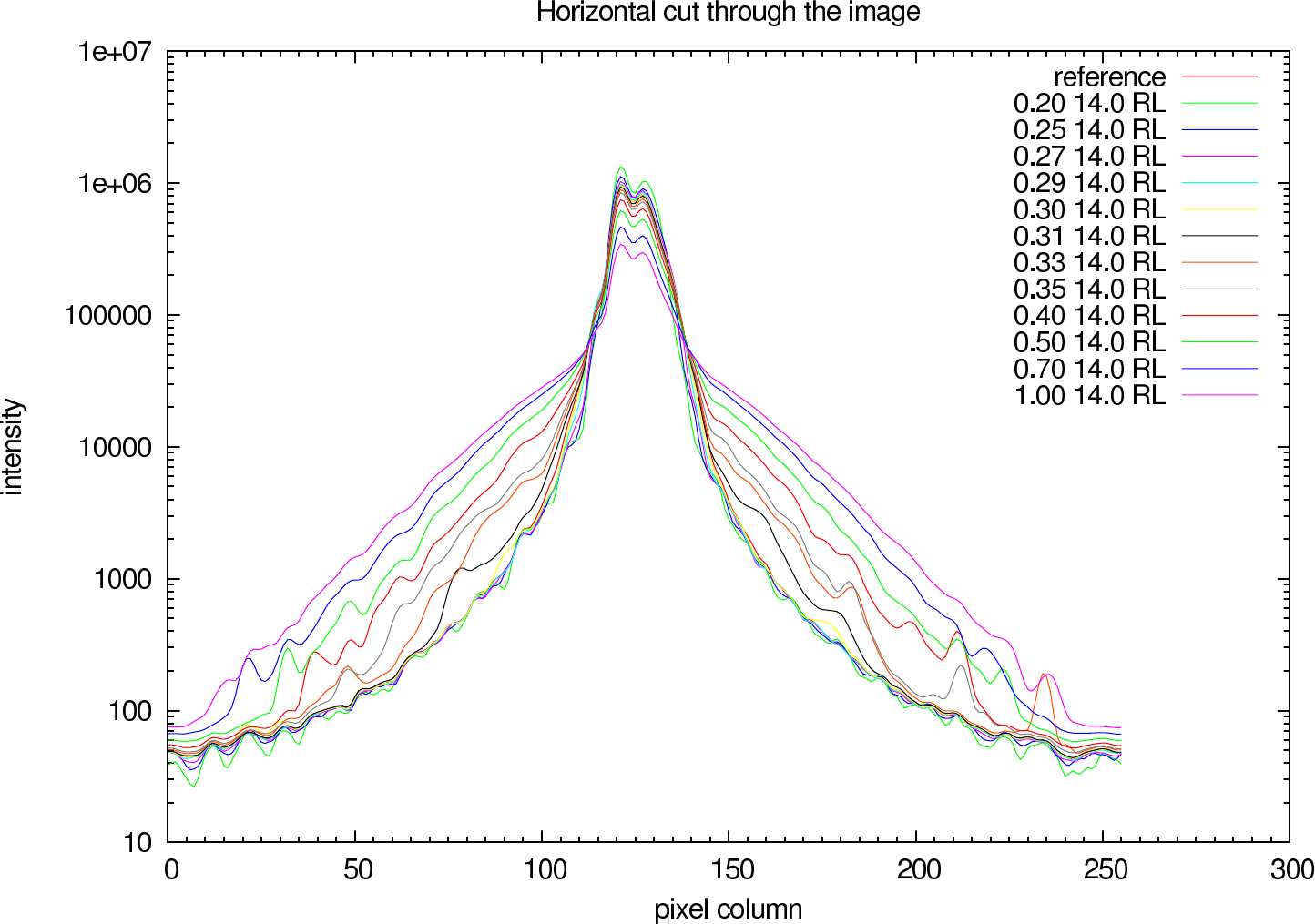
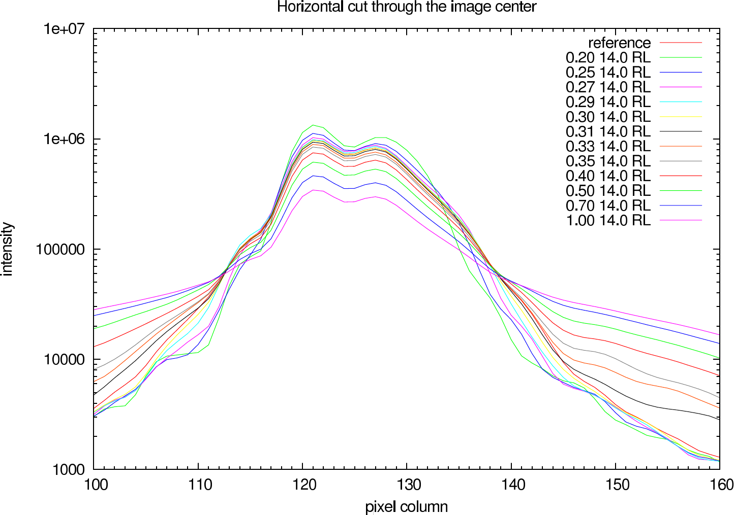
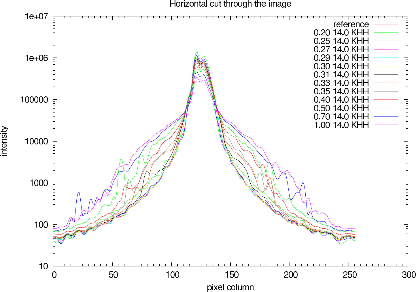
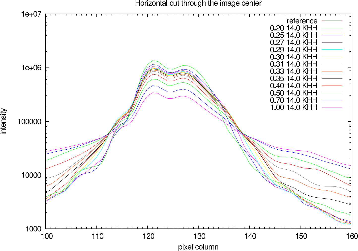
In figure 8 (J-Band) and figure 9 (K-Band) a horizontal cut slightly above the intensity maximum of the reconstructions of NHC4151 compared with the ideal reference image is shown.

Figure 8: Horizontal profile through the center of the reconstructed galaxy compared to the ideal image (J-Band). On the right side only the central part is shown. In the first row, Richardson-Lucy was used for the reconstruction. In the second row, the Building-Block method was used.

Figure 9: Horizontal profile through the center of the reconstructed galaxy compared to the ideal image (K-Band). On the right side only the central part is shown. In the first row, Richardson-Lucy was used for the reconstruction. In the second row, the Building-Block method was used.

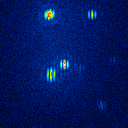
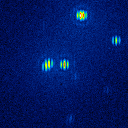
The basis of this simulation is a small star cluster (see figure 2). The simulated raw images are shown in figure 10.

Figure 10: The simulated raw images for position angles of 108, 144, 180, 216, and 252 degree of a star cluster including sky background (top row J-Band, bottom row K-Band).

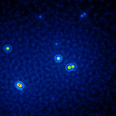
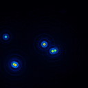
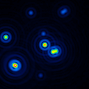
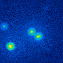
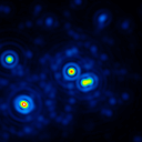
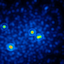
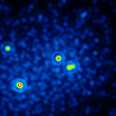
A comparison of the reconstructions depending on the calibrator strehl is presented in figure 11 (J-Band) and figure 12 (K-Band).

Figure 11: Star cluster: The J-Band reconstructions depending on the calibrator strehl are shown in this figure. The top left image shown the reference image of the star cluster. The top right image shown the five coadded raw images. The second row show the reconstructions using the Richardson-Lucy algorithm. The calibrator strehl was 0.20, 0.30 (same as for the target), 0.40, and 1.0 (from left to right). In the third row, the Building-Block algorithm was used.

Figure 12: Star cluster: The K-Band reconstructions depending on the calibrator strehl are shown in this figure. The top left image shown the reference image of the star cluster. The top right image shown the five coadded raw images. The second row show the reconstructions using the Richardson-Lucy algorithm. The calibrator strehl was 0.20, 0.30 (same as for the target), 0.40, and 1.0 (from left to right). In the third row, the Building-Block algorithm was used.

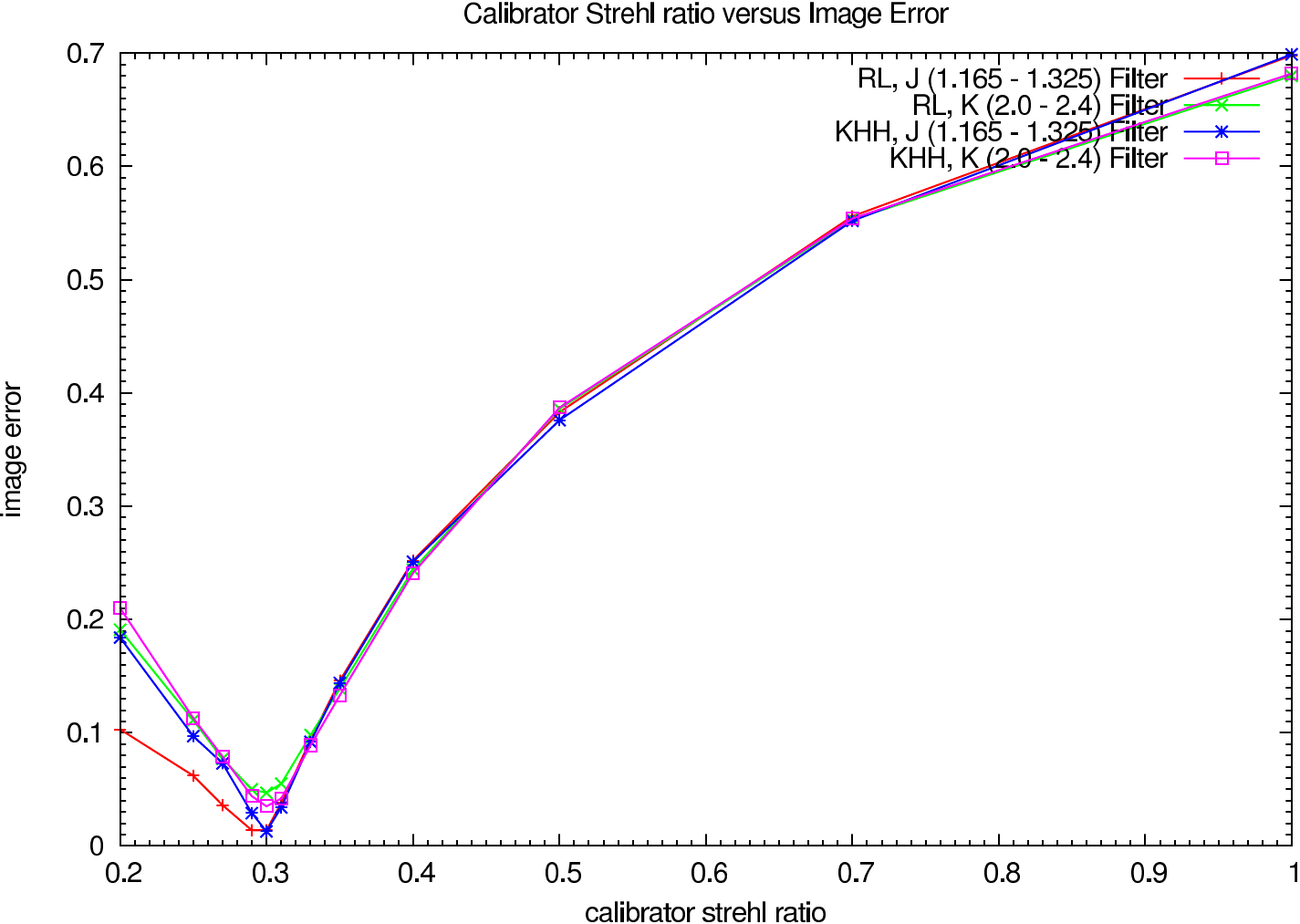
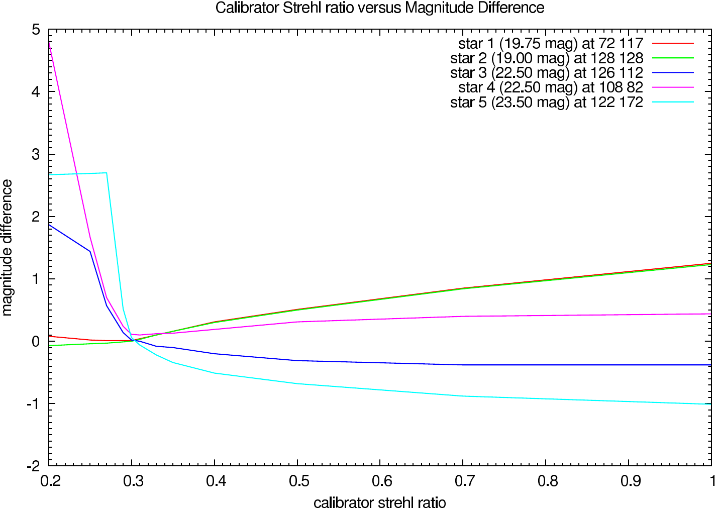
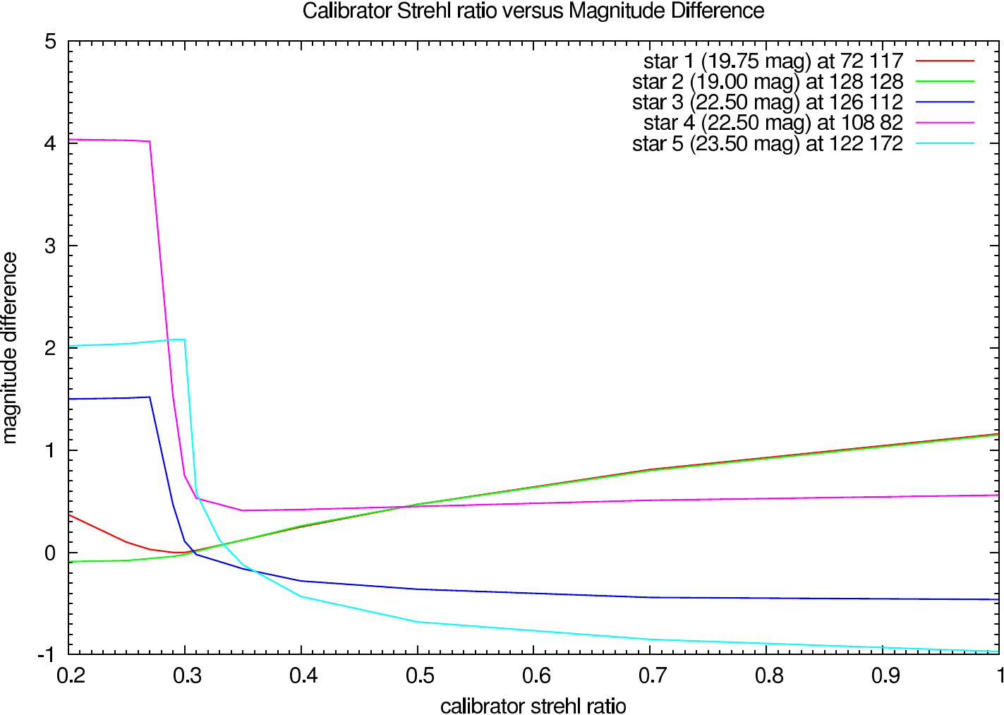
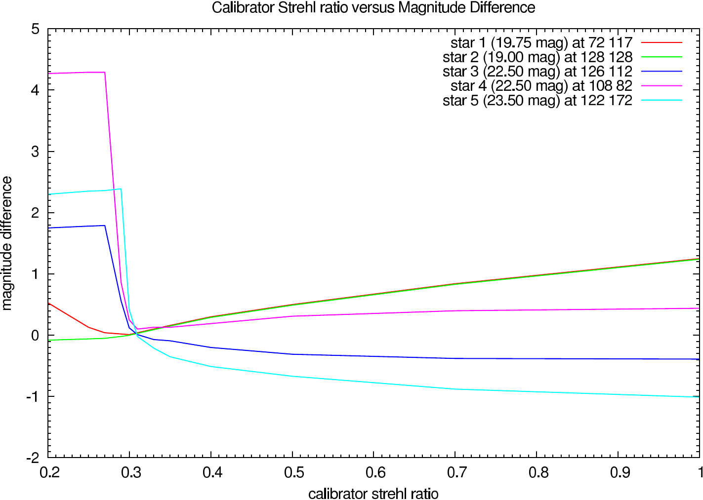
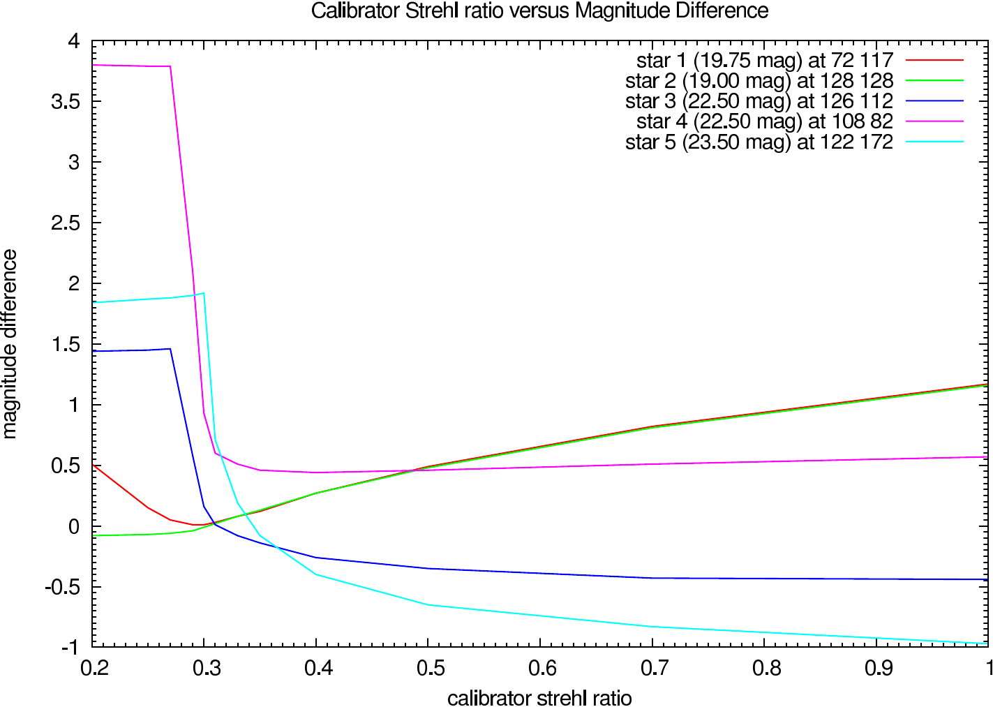
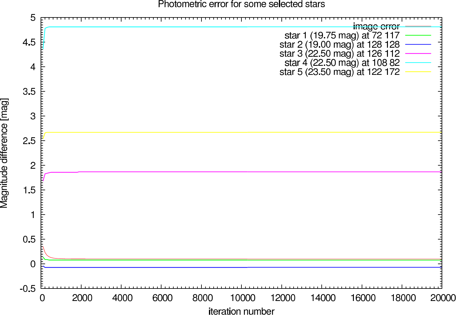
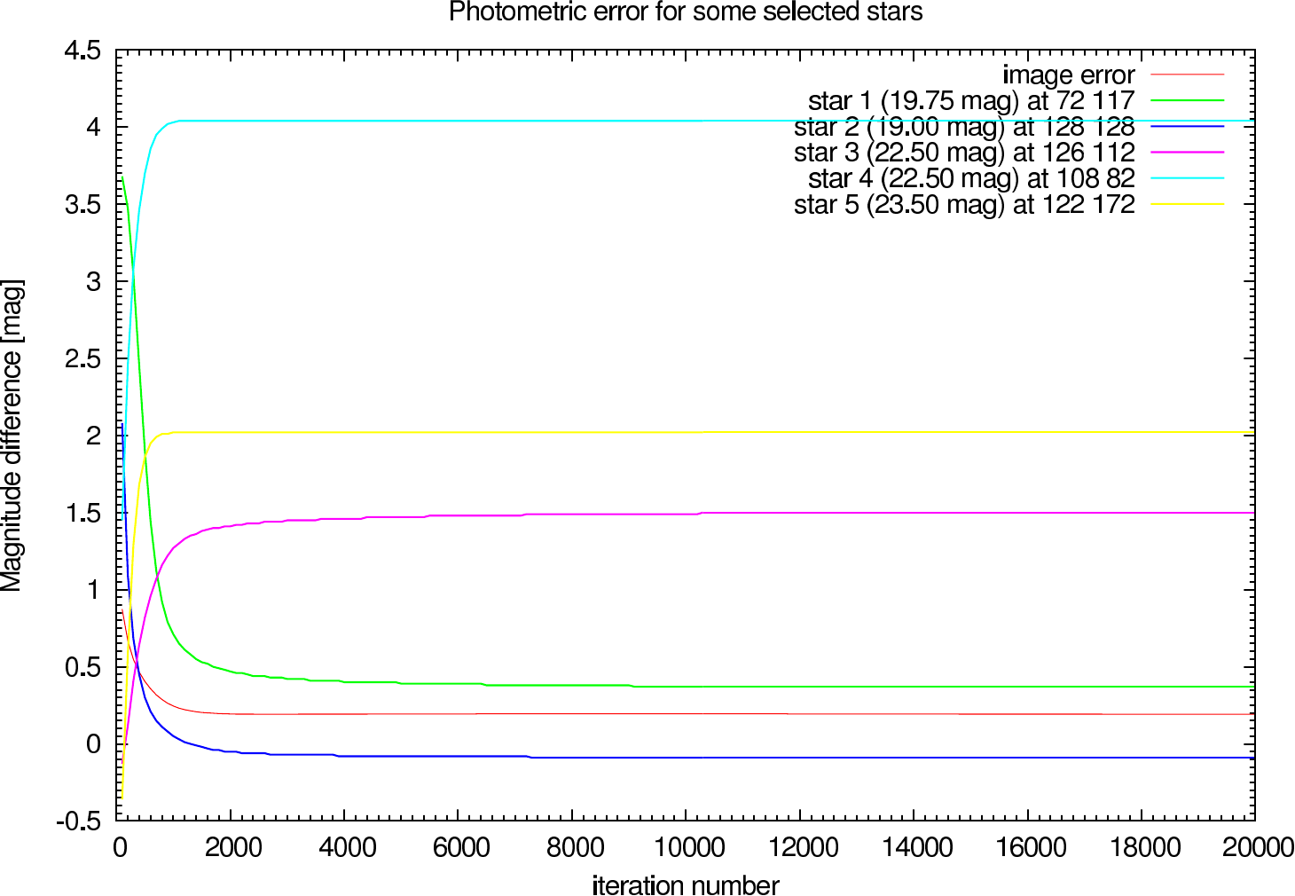
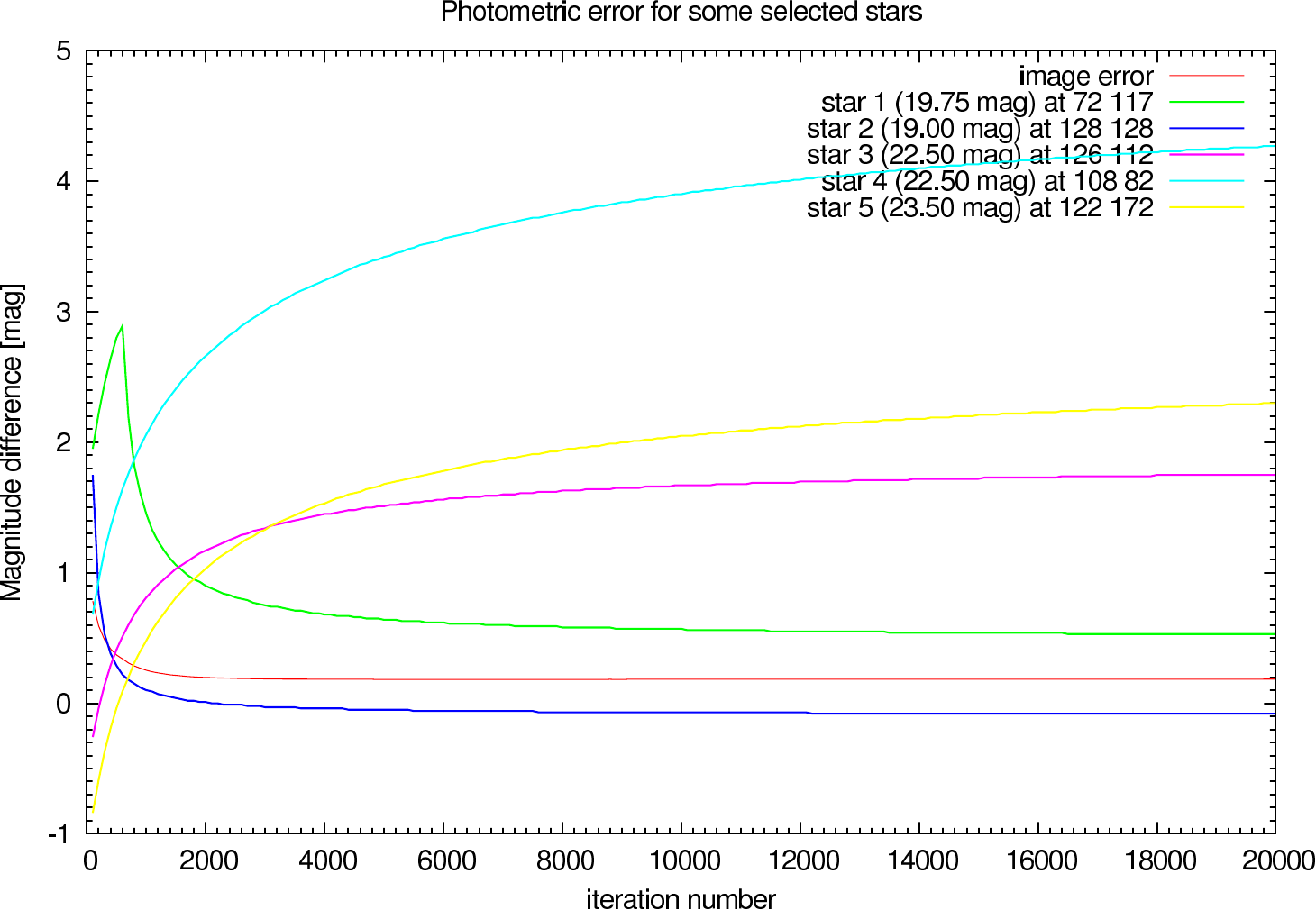
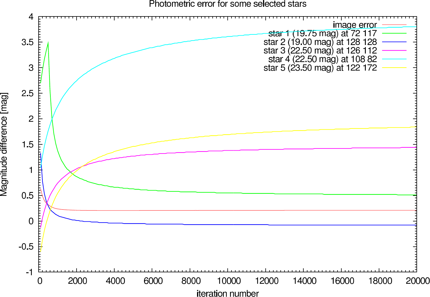
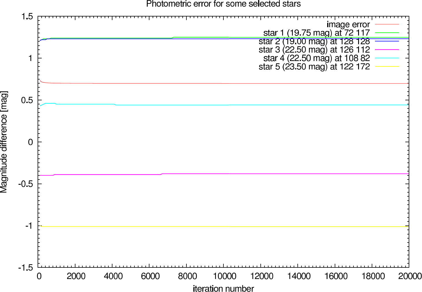
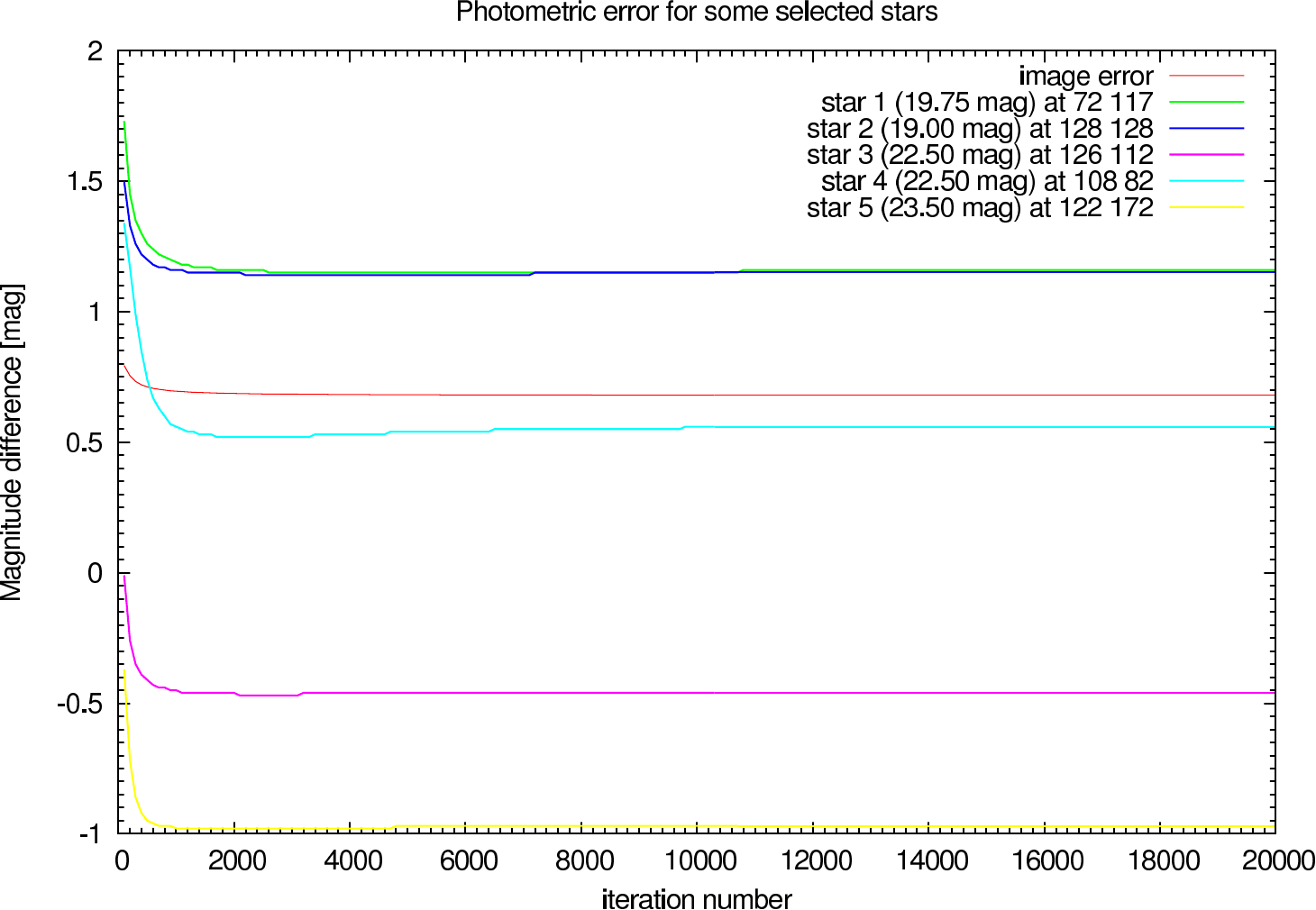
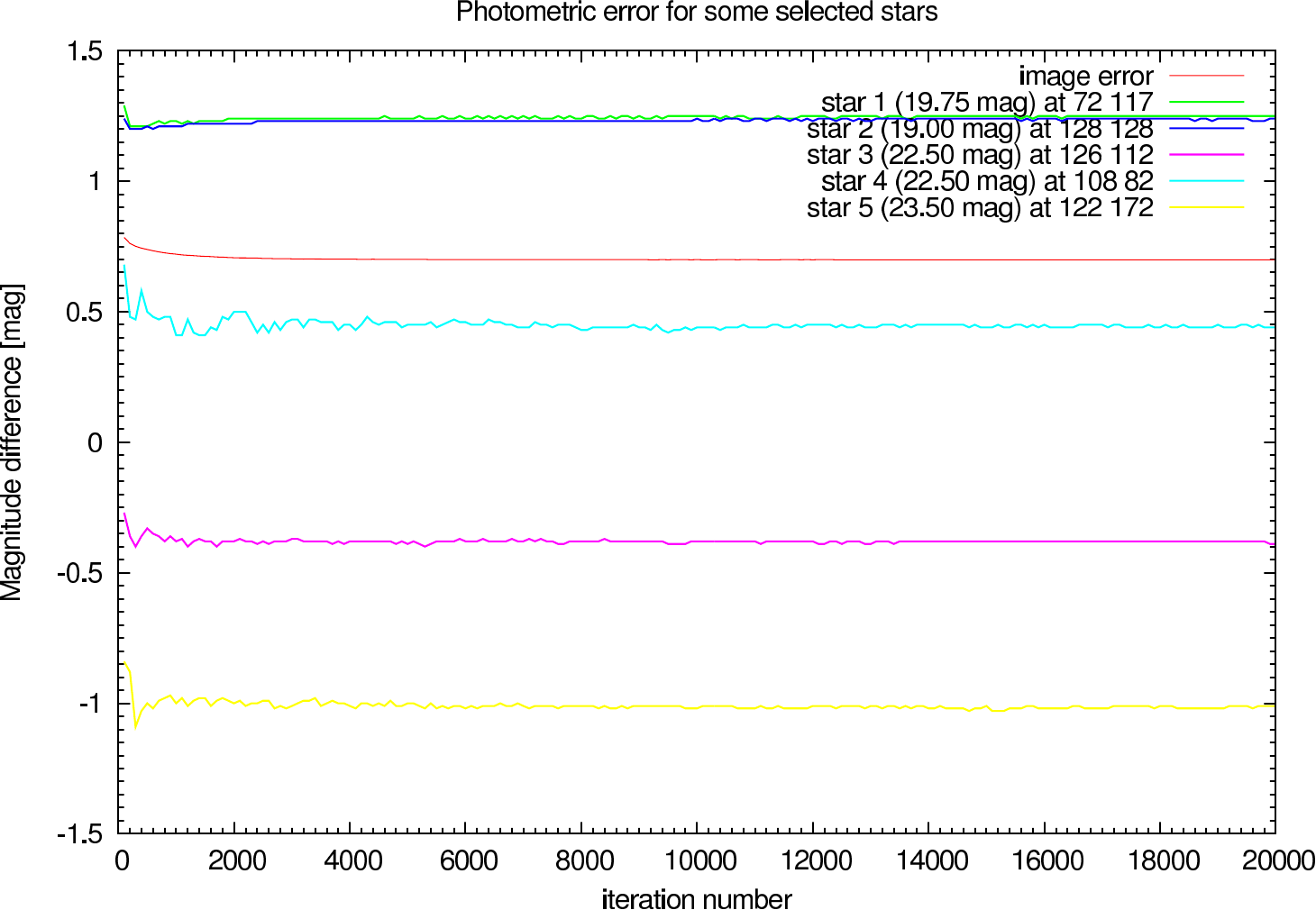
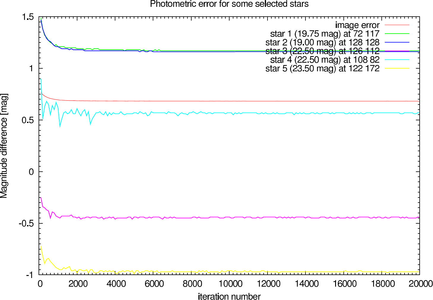
In table 4 (J-Band) and table 5 (K-Band) the errors for the star cluster depending on the calibrator strehl are presented.. The image errors are also summarized in figure 13 and the photometric errors in figure 14.

Figure 13: In this figure, the image errors depending on the calibrator strehl ratio are shown.

Figure 14: Photometric errors depending on the calibrator strehl ratio in the J-Band (left side) and K-Band (right side). The reconstruction in the first row uses the Richardson-Lucy algorithm, in the second row, the Building-Block method was used.

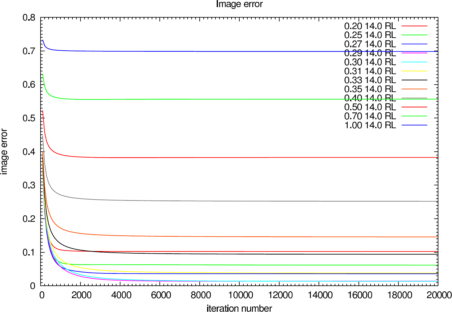
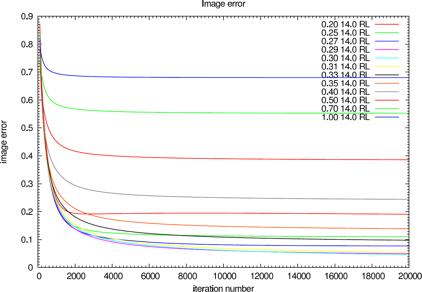
In figure 15 the image error describing the difference between the reconstruction and the reference image is shown for each iteration (in steps of 100 iterations). The effect of the calibrator strehl on the reconstruction error and the optimal iteration number is clearly visible.

Figure 15: Reconstruction error depending on the iteration number for the J-Band (left side) and K-Band (right side). In the first row, Richardson-Lucy was used for the reconstruction. In the second row, the Building-Block method was used.

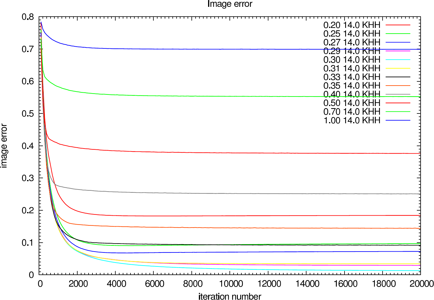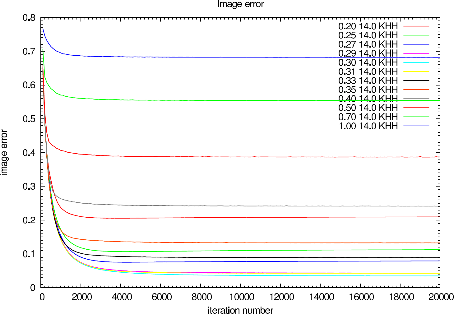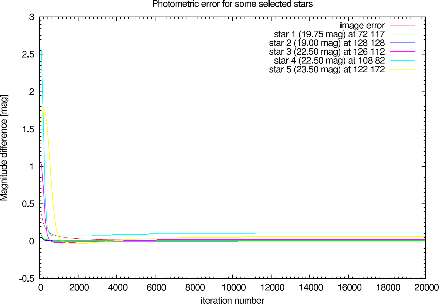
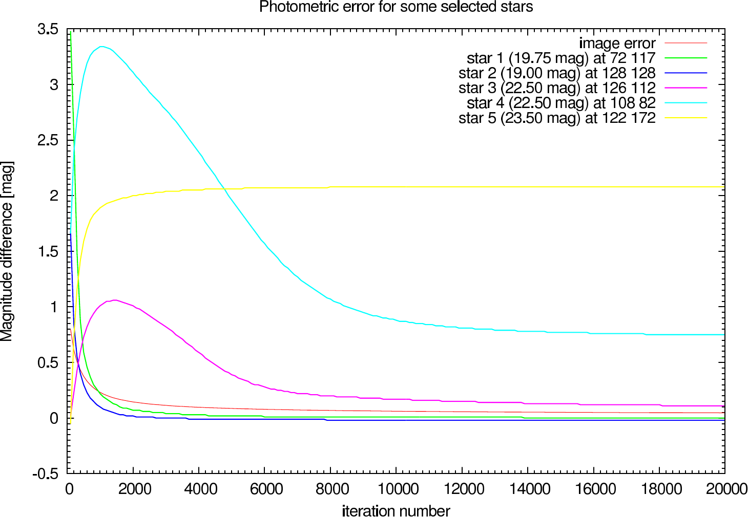
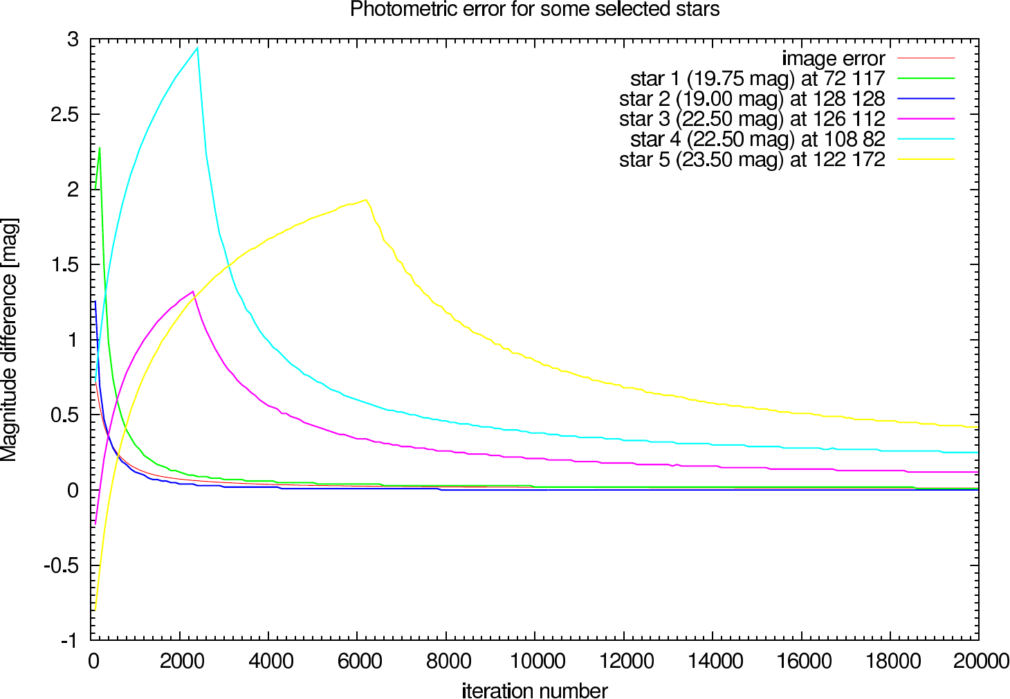
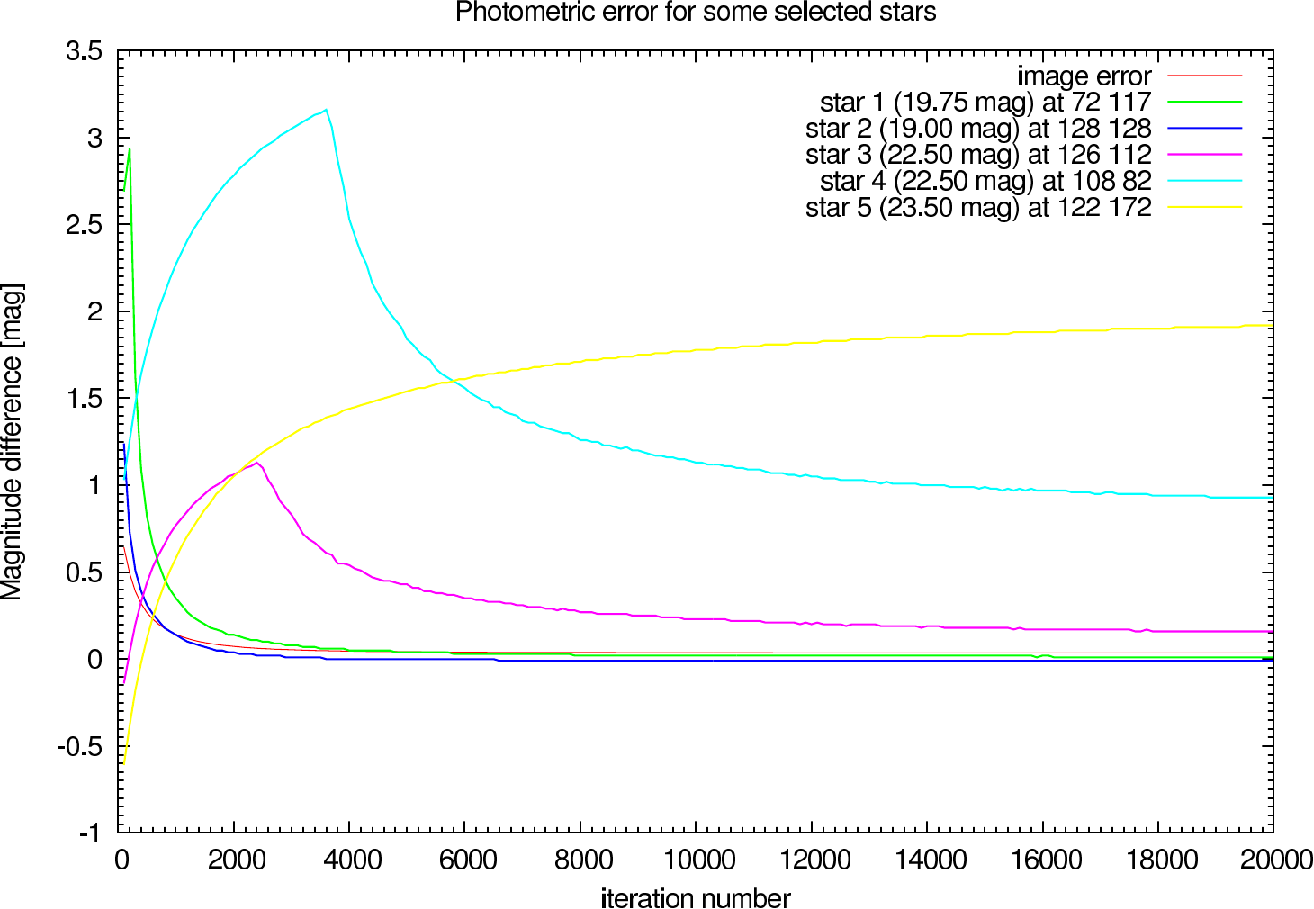
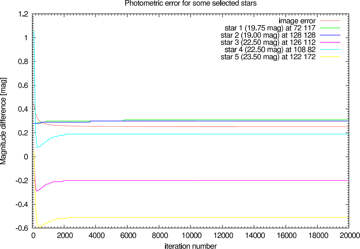
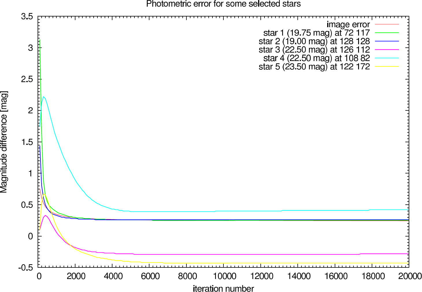
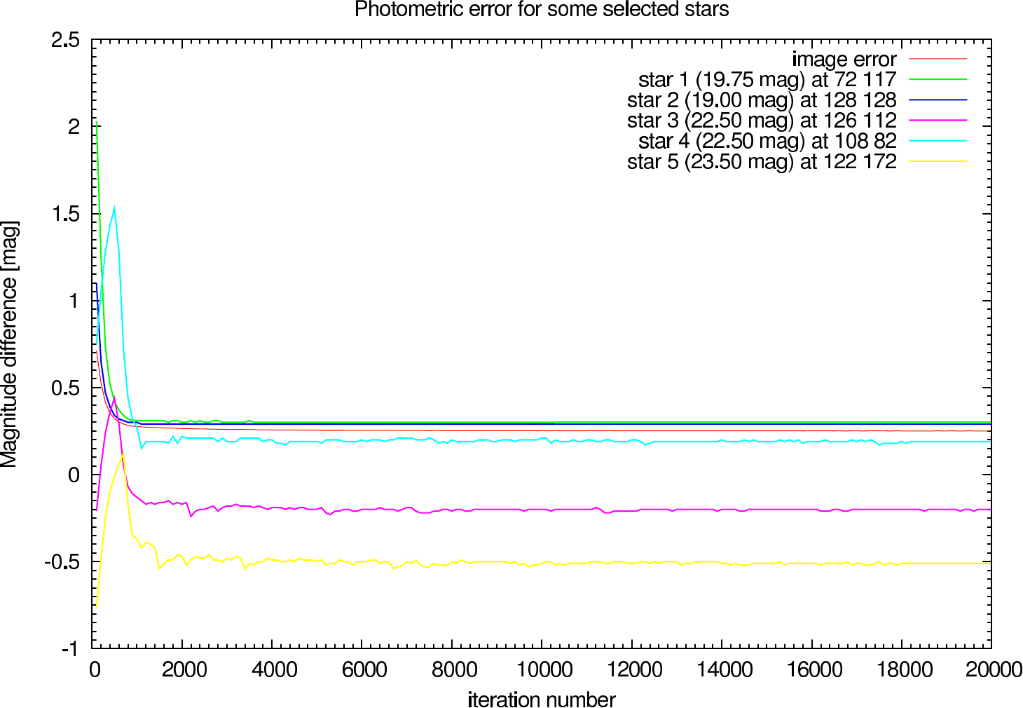
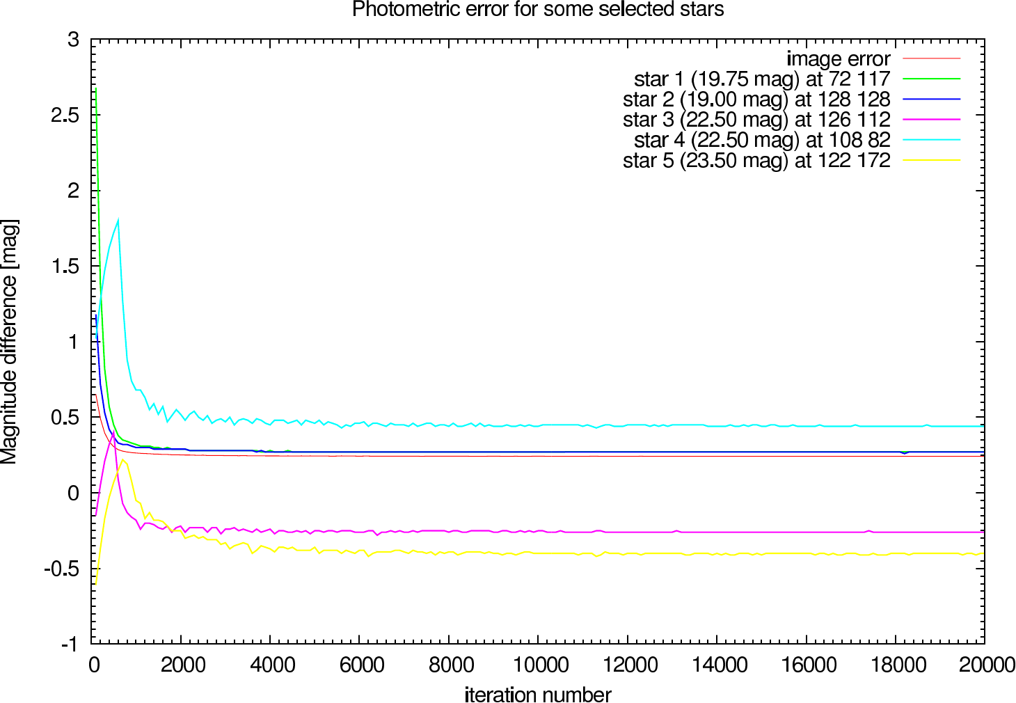
In the figures figure , figure 16, figure 17, figure 18, and figure 19 the image and photometric errors depending on the calibrator strehl and the iteration number is shown. The overall shape is the same, but the optimum number of iterations is difficult to select, because not all photometric errors have their minimum at the same iteration number.

Figure 16: Image and photometric errors depending on the iteration number in the J-Band (left side) and K-Band (right side). The calibrator has a strehl of 0.20. In the first row, Richardson-Lucy was used for the reconstruction. In the second row, the Building-Block method was used.

Figure 17: Image and photometric errors depending on the iteration number in the J-Band (left side) and K-Band (right side). The calibrator has a strehl of 0.30. In the first row, Richardson-Lucy was used for the reconstruction. In the second row, the Building-Block method was used.

Figure 18: Image and photometric errors depending on the iteration number in the J-Band (left side) and K-Band (right side). The calibrator has a strehl of 0.40. In the first row, Richardson-Lucy was used for the reconstruction. In the second row, the Building-Block method was used.

Figure 19: Image and photometric errors depending on the iteration number in the J-Band (left side) and K-Band (right side). The calibrator has a strehl of 1.00. In the first row, Richardson-Lucy was used for the reconstruction. In the second row, the Building-Block method was used.