This simulation should give an answer to the question how the quality of the reconstruction depends on the magnitude of a calibrator. The difficulties arising from a non constant sky background due to an object halo, or an imperfect AO are ignored. The setup used for this experiment is (for the common test setup see table 1):

• This experiment uses monochromatic PSFs for the J- and K-Band with a strehl of 0.3. In contrast to all other simulations the calibrator and target uses the same PSF.
• The AO delivers a strehl of about 30 percent.
• In order to test the sensitivity to the calibrator brightness, magnitudes from 14mag to 22 mag in 1mag steps are used.
• Two different targets were used:
  1. A scaled down image of NGC4151 and an overlayed image of a simulated dust torus (AGN).
  2. A small star cluster where different distances and brightness levels do exist
• For each position angle (108, 144, 180, 216, 252 degree) an image equivalent to 60 seconds exposure time was created.

This experiment uses monochromatic PSFs for the J- and K-Band with a strehl of 0.3. In contrast to all other simulations the calibrator and target uses the same PSF. Therefore only the brightness of the target and calibrator has an influence on the deconvolution. The setup for the PSF generation is described in table 1.

The experiment uses a target which consists of a scaled down image of NGC4151 and an overlayed image of a simulated dust torus. A second object shows a small star cluster where different distances and brightness levels do exist. These objects are observed (we assume this) in J-Band and K-band five times at different position angles. The image contains exactly one star which can be used as a calibrator. It was additionally assumed, that the background around this star could be perfectly compensated (no inhomogenious sky background or target halo).

The raw data were generated according to the common scheme described in section Overview. In addition, the images for the target and calibrator are generated separately which means, that the psf-star image is not influenced by the target (no halo, etc.).

All simulated input data for the LN DRS pipeline are available as tar-files (ex1_j_input.tar.gz (16MB) and ex1_k_input.tar.gz (18MB)). The corresponding results are also available as tar files (ex1_j_results.tar.gz (4.8MB) and ex1_k_results.tar.gz (5.2MB)).

The generated calibrator raw images are shown in section Calibrator. The raw images and deconvolution results are shown in section Raw Frames and Results for an AGN for the AGN and section Raw Frames and Results for a Star Cluster for the star cluster.

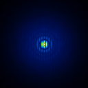
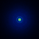
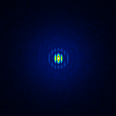
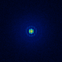
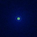
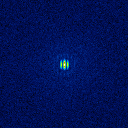
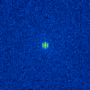
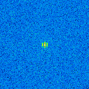
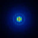
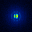
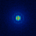
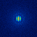
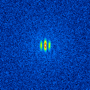
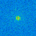
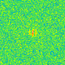
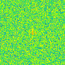
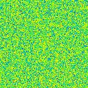
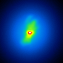
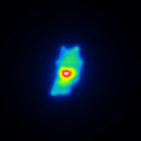
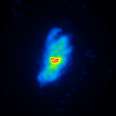
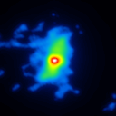
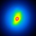
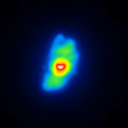
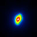
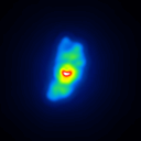
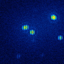
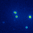
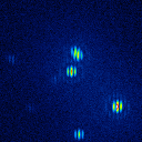
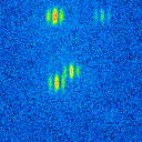
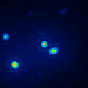
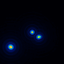
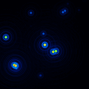
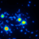
The simulated raw LBT interferograms used for the deconvolution are ideal images, they are not influenced by detector effects like different pixel gain or bad pixels. In figure 1 (J-Band) and figure 2 (K-Band) the psf-stars for some stellar brightness levels are shown.

Figure 1: Central 128x128 pixels of the generated J-Band images of a calibrator at different magnitudes (from top left to bottomright: 14, 15, 16, 17, 18, 19, 20, 21, and 22mag).

Figure 2: Central 128x128 pixels of the generated K-Band images of a calibrator at different magnitudes (from top left to bottomright: 14, 15, 16, 17, 18, 19, 20, 21, and 22mag).

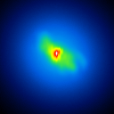
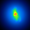
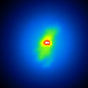
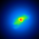
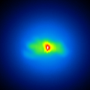
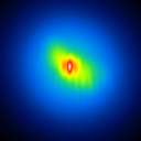
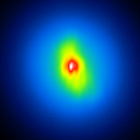
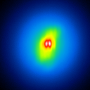
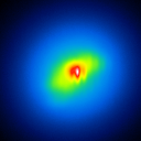
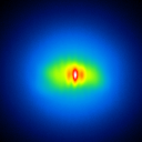
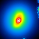
The basis of this simulation is an image of NGC4151 with an overlayed dust torus (see figure 1). The simulated raw images are shown in figure 3.

Figure 3: The simulated raw images for position angles of 108, 144, 180, 216, and 252 degree of NGC4151 at 10.1mag including sky background (top row J-Band, bottom row K-Band).

A comparison of the reconstructions depending on the calibrator brightness is presented in figure 4 (J-Band) and figure 5 (K-Band).

Figure 4: AGN: The J-Band reconstructions depending ion the calibrator brightness are shown in this figure. The top left image shown the reference image of NGC4151. The top right image shown the five coadded raw images. The second row show the reconstructions using the Richardson-Lucy algorithm. The calibrator brightness was 14 mag, 18 mag, and 22 mag (from left to right). In the third row, the Building-Block algorithm was used.

Figure 5: AGN: The K-Band reconstructions depending ion the calibrator brightness are shown in this figure. The top left image shown the reference image of NGC4151. The top right image shown the five coadded raw images. The second row show the reconstructions using the Richardson-Lucy algorithm. The calibrator brightness was 14 mag, 18 mag, and 22 mag (from left to right). In the third row, the Building-Block algorithm was used.

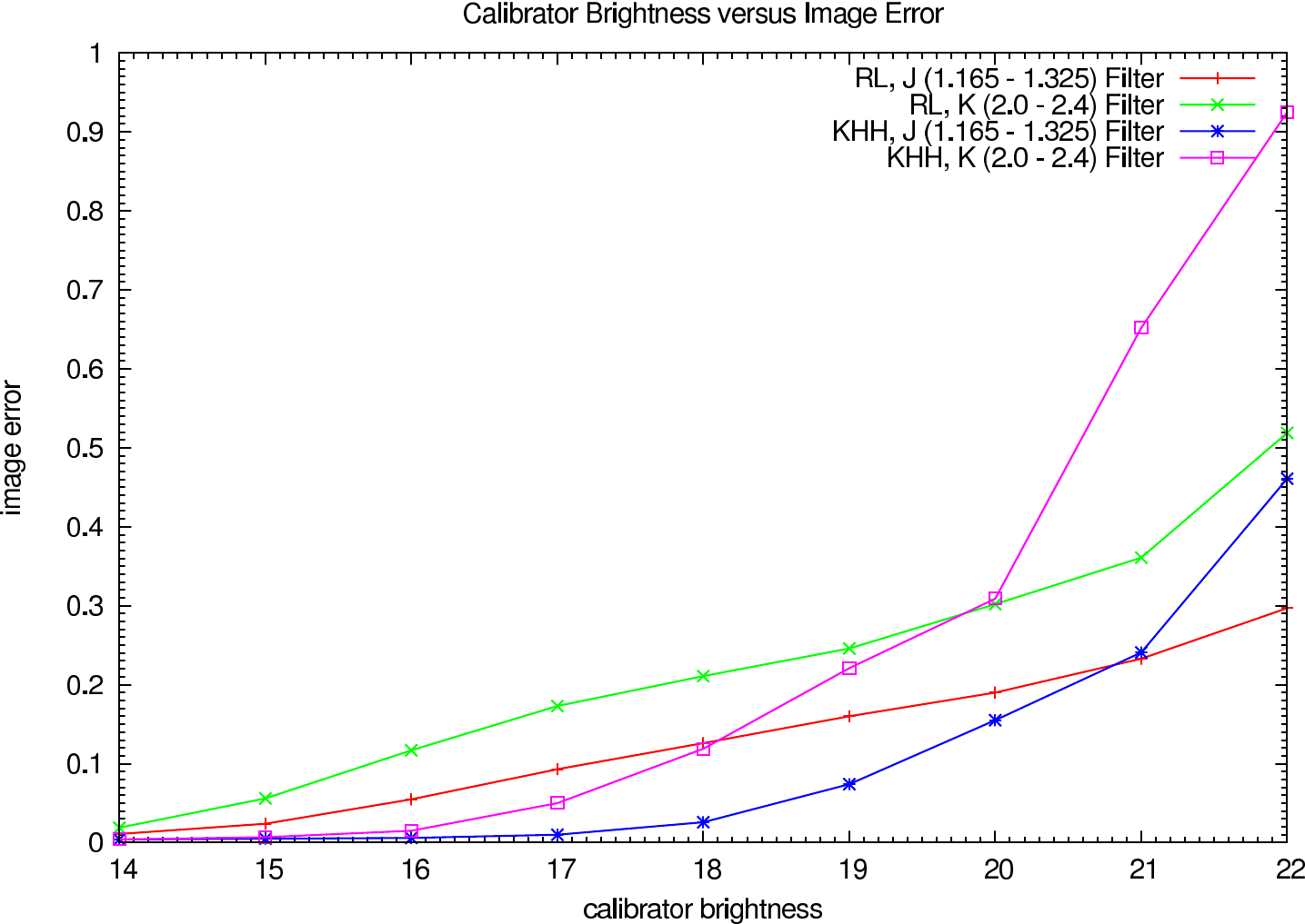
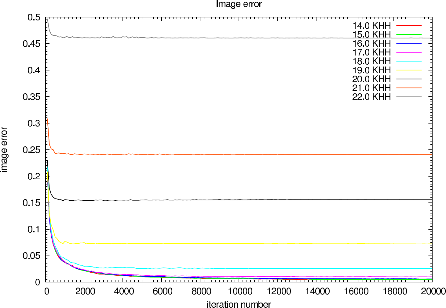
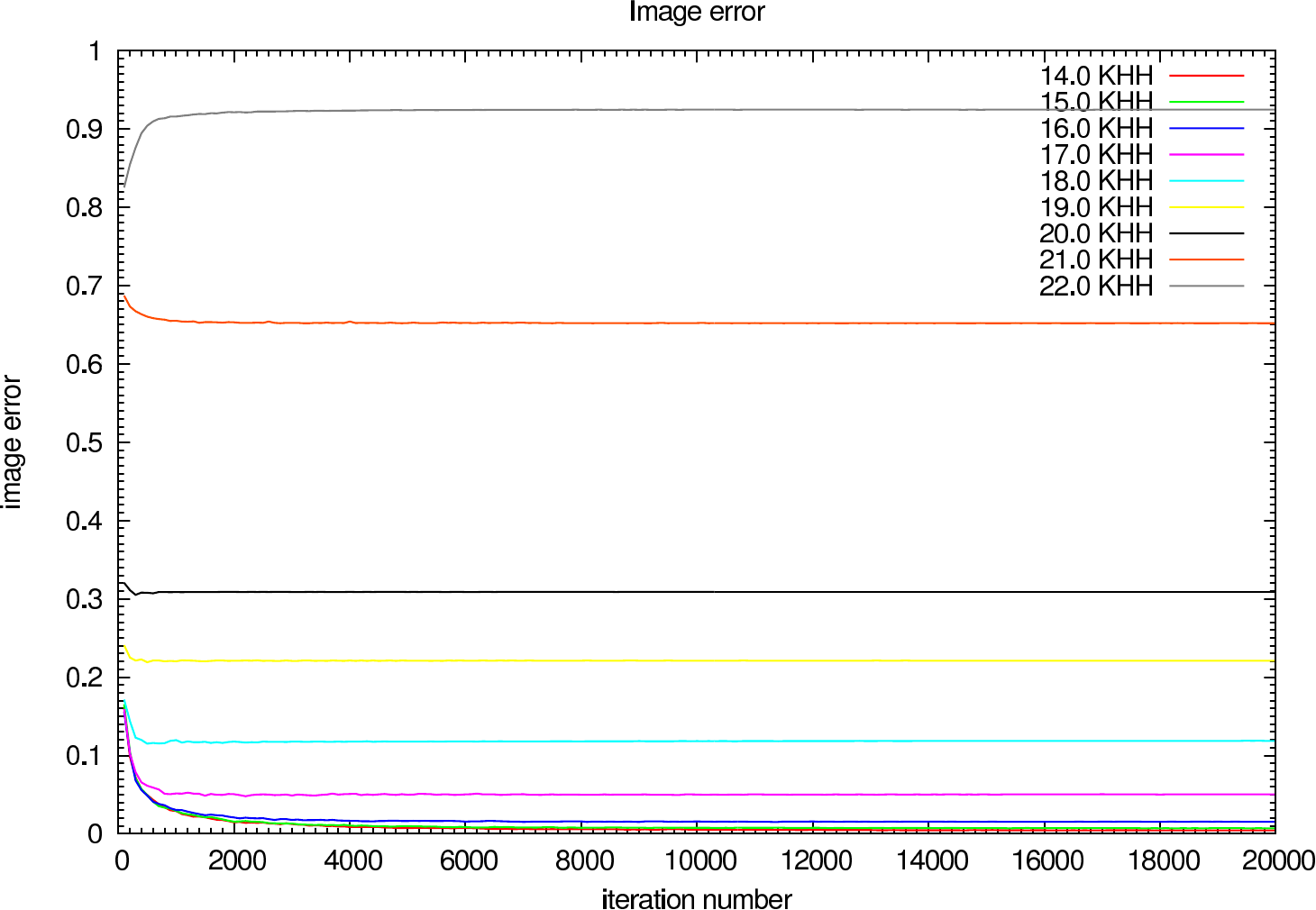
In table 2 (J-Band) and table 3 (K-Band) the errors for the AGN depending on the psf star brightness are presented. In figure 6 the image errors depending on the calibrator brightness are shown.

Figure 6: In this figure, the image errors depending on the calibrator brightness are shown.

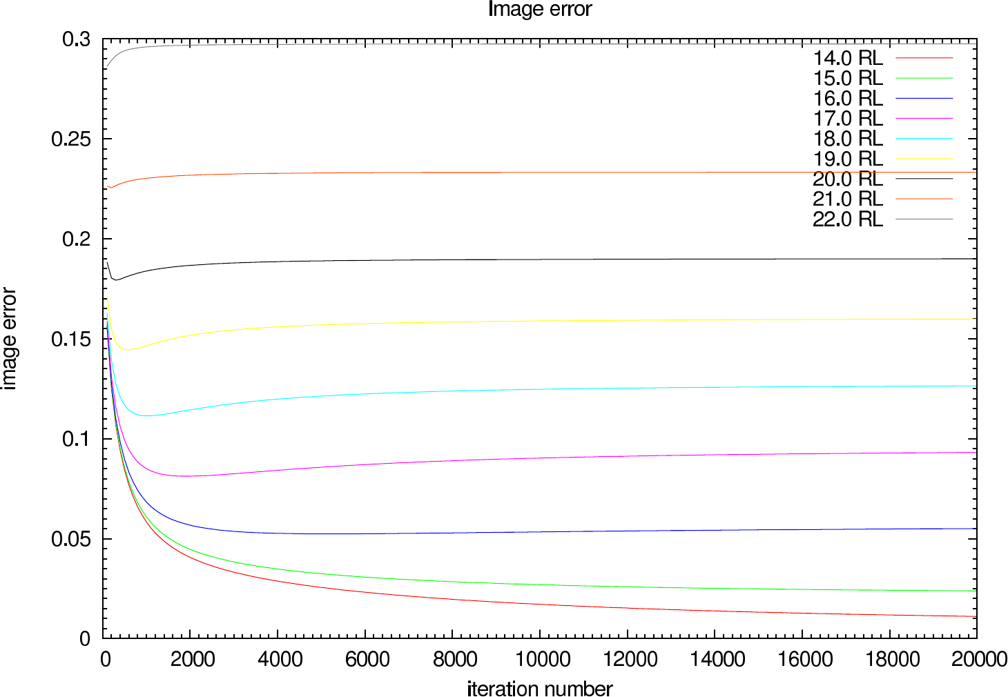
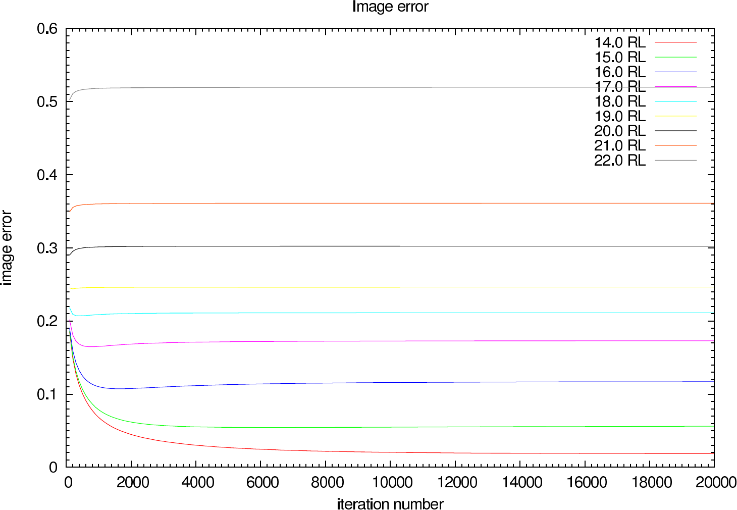
In figure 7 the image error describing the difference between the reconstruction and the reference image is shown for each iteration (in steps of 100 iterations). The effect of the calibratior brightness on the reconstruction error and the optimal iteration number is clearly visible.

Figure 7: Reconstruction error depending on the iteration number for the J-Band (left side) and the K-Band (right side). The reconstruction in the first row uses the Richardson-Lucy algorithm, in the second row, the Building-Block method was used.

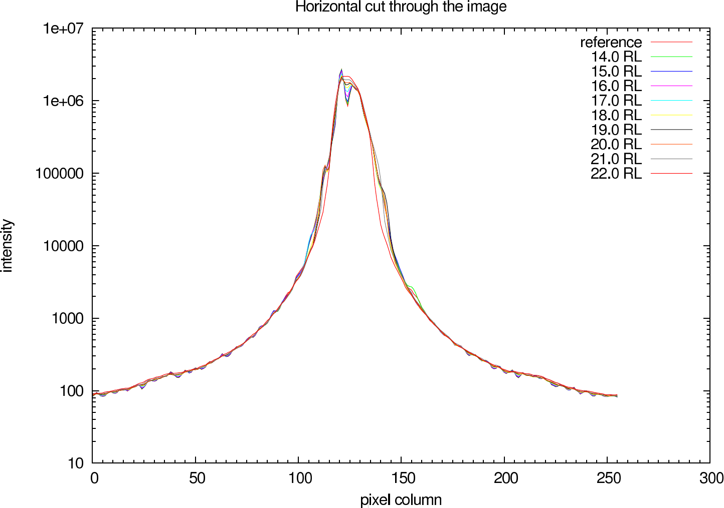
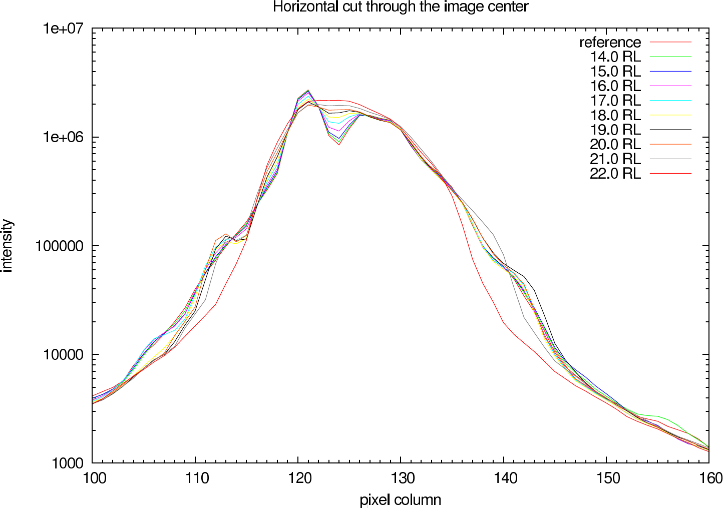
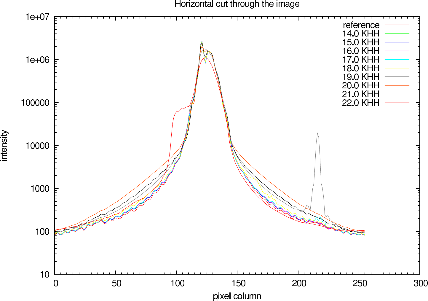
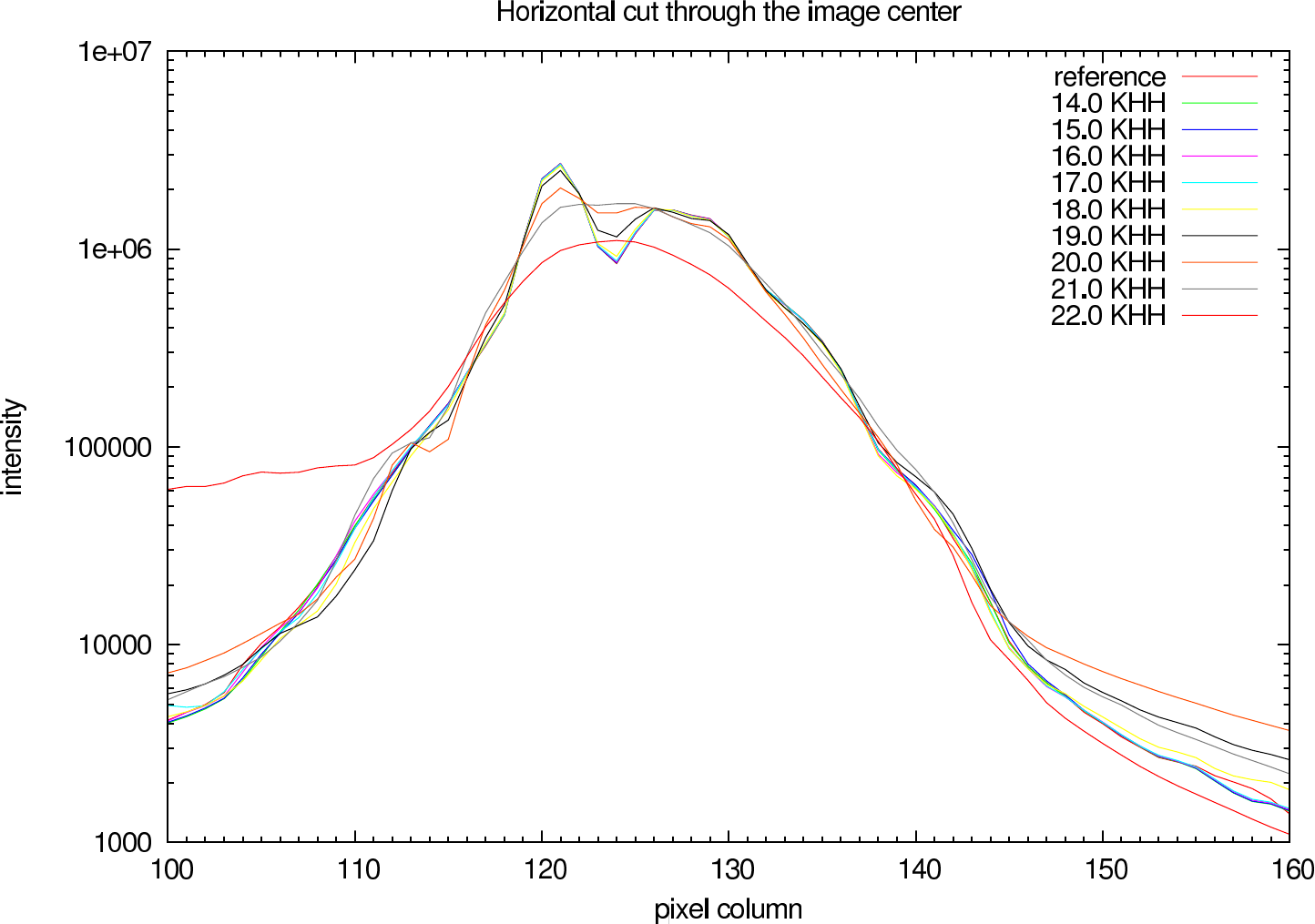
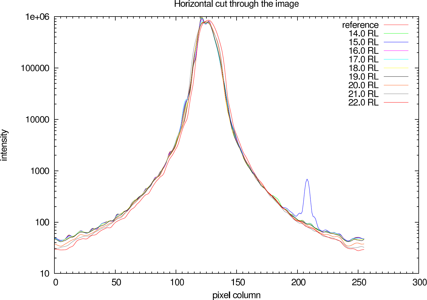
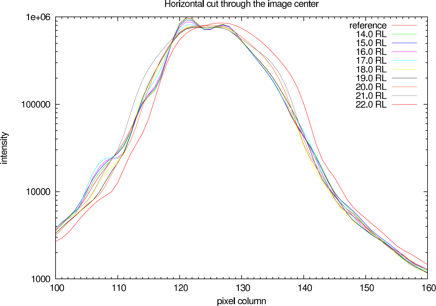
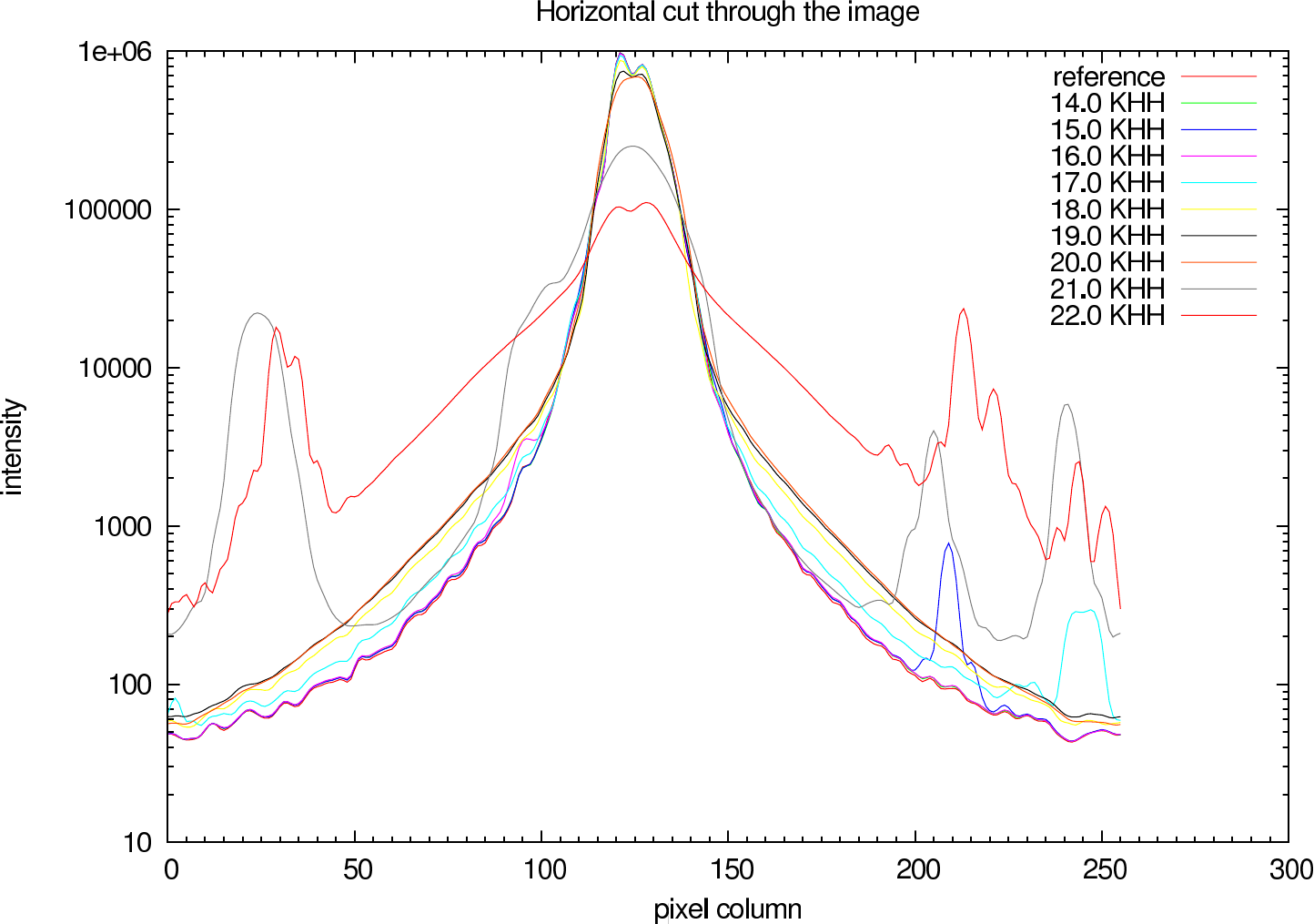
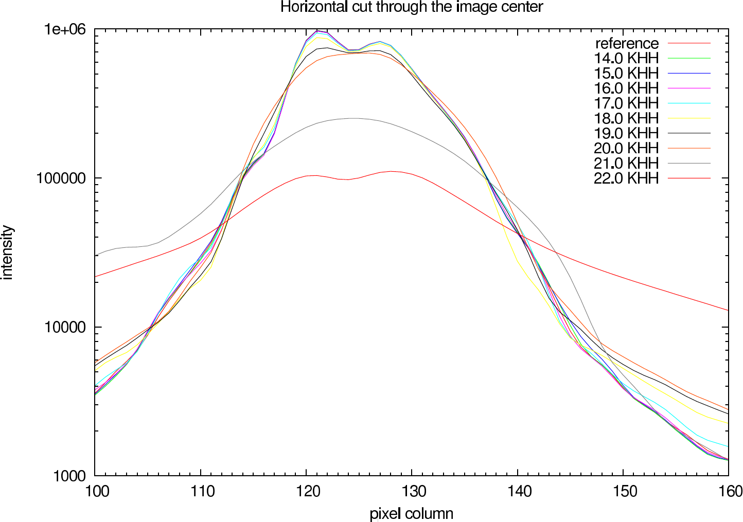
In figure 8 (J-Band) and figure 9 (K-Band) a horizontal cut slightly above the intensity maximum of the reconstructions of NGC4151 compared with the ideal reference image is shown.

Figure 8: Horizontal profile through the center of the reconstructed galaxy compared to the ideal image (J-Band). On the right side only the central part is shown. The reconstruction in the first row uses the Richardson-Lucy algorithm, in the second row, the Building-Block method was used.

Figure 9: Horizontal profile through the center of the reconstructed galaxy compared to the ideal image (K-Band). On the right side only the central part is shown. The reconstruction in the first row uses the Richardson-Lucy algorithm, in the second row, the Building-Block method was used.

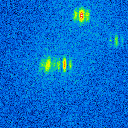
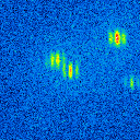
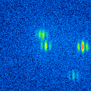
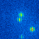
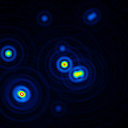
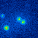
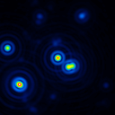
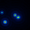
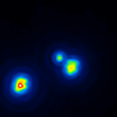
The basis of this simulation is a small star cluster (see figure 2). The simulated raw images are shown in figure 10.

Figure 10: The simulated raw images for position angles of 108, 144, 180, 216, and 252 degree of a star cluster including sky background (top row J-Band, bottom row K-Band).

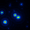
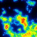
A comparison of the reconstructions depending on the calibrator brightness is presented in figure 4 (J-Band) and figure 5 (K-Band).

Figure 11: Star cluster: The J-Band reconstructions depending ion the calibrator brightness are shown in this figure. The top left image shown the reference image of the star cluster. The top right image shown the five coadded raw images. The second row show the reconstructions using the Richardson-Lucy algorithm. The calibrator brightness was 14 mag, 18 mag, and 22 mag (from left to right). In the third row, the Building-Block algorithm was used.

Figure 12: Star cluster: The K-Band reconstructions depending ion the calibrator brightness are shown in this figure. The top left image shown the reference image of the star cluster. The top right image shown the five coadded raw images. The second row show the reconstructions using the Richardson-Lucy algorithm. The calibrator brightness was 14 mag, 18 mag, and 22 mag (from left to right). In the third row, the Building-Block algorithm was used.

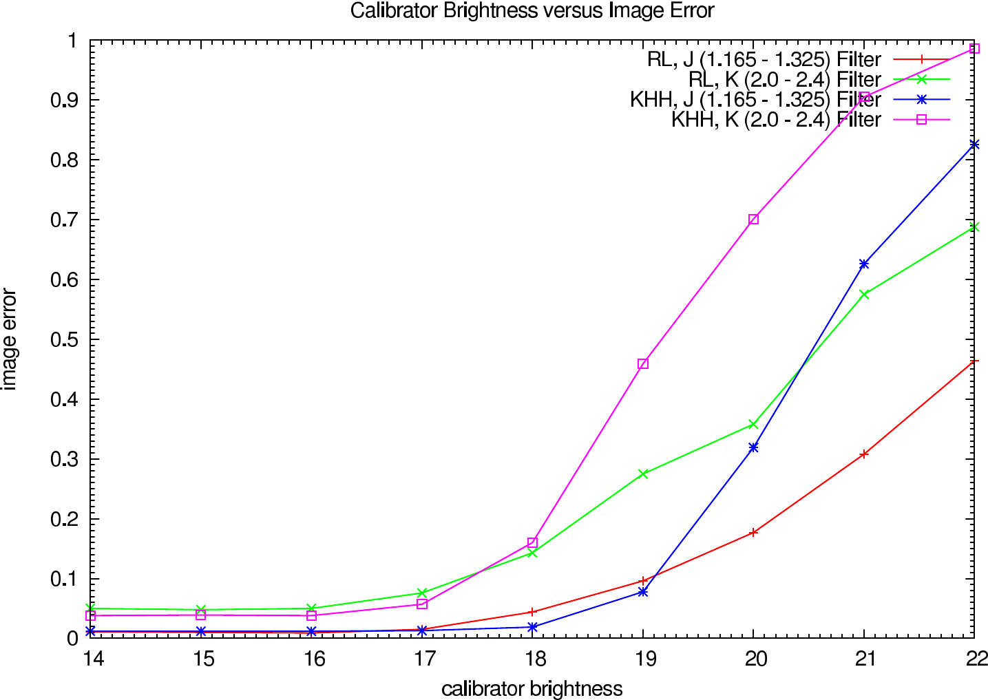
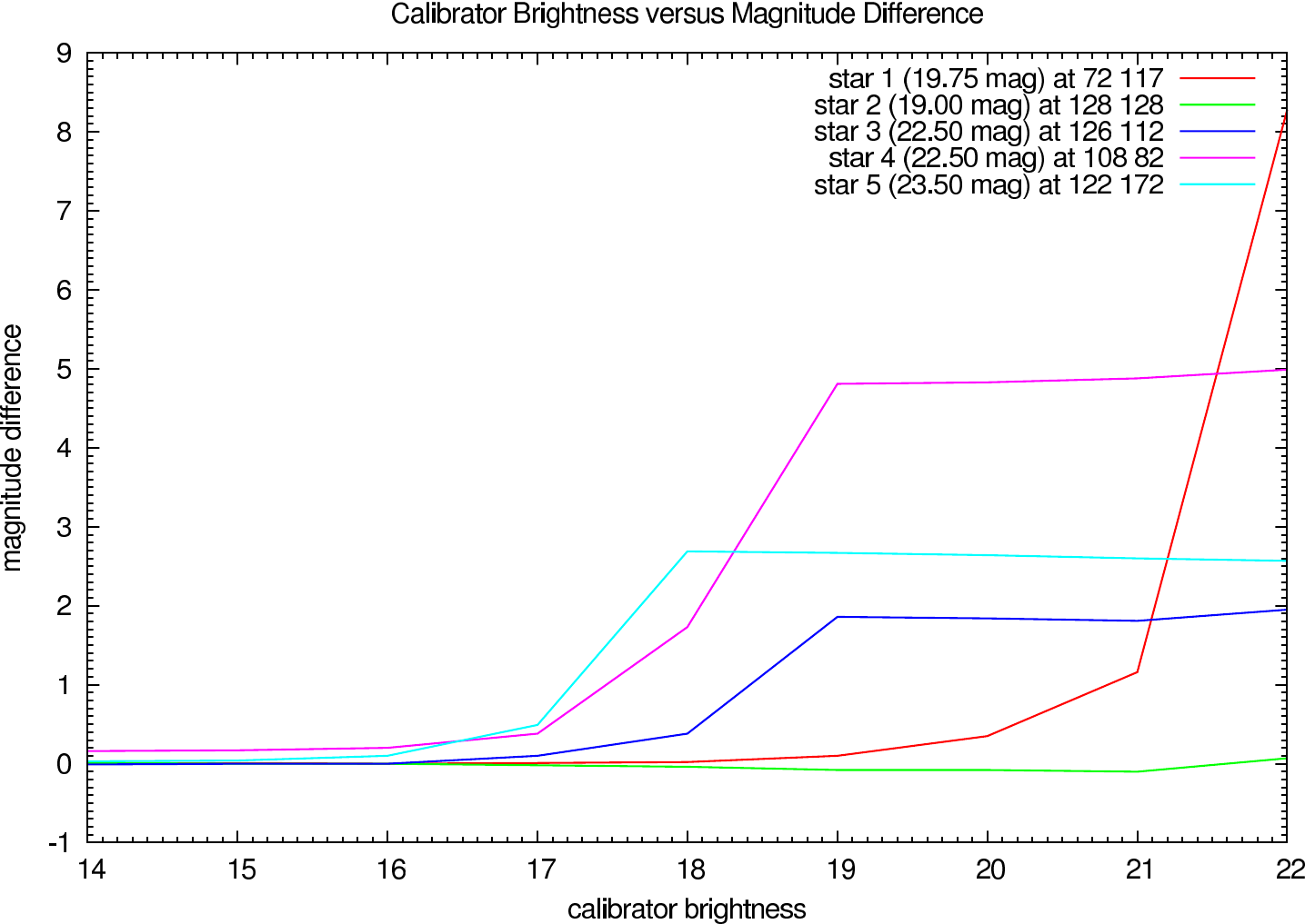
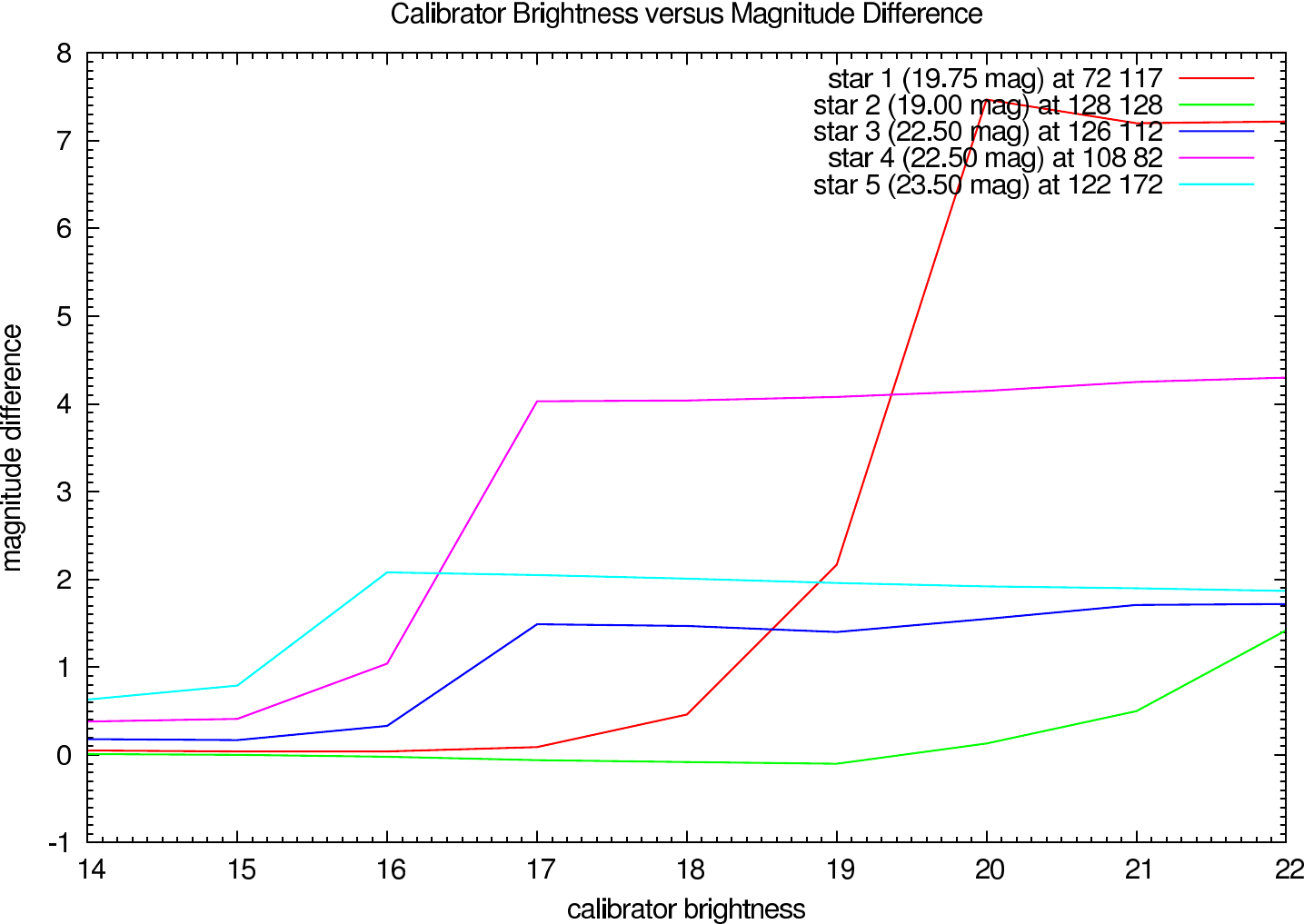
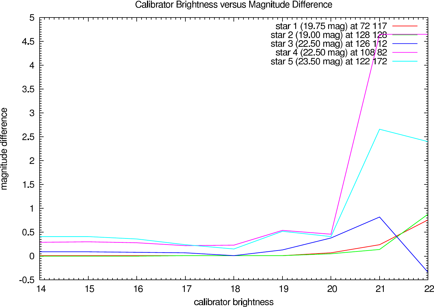
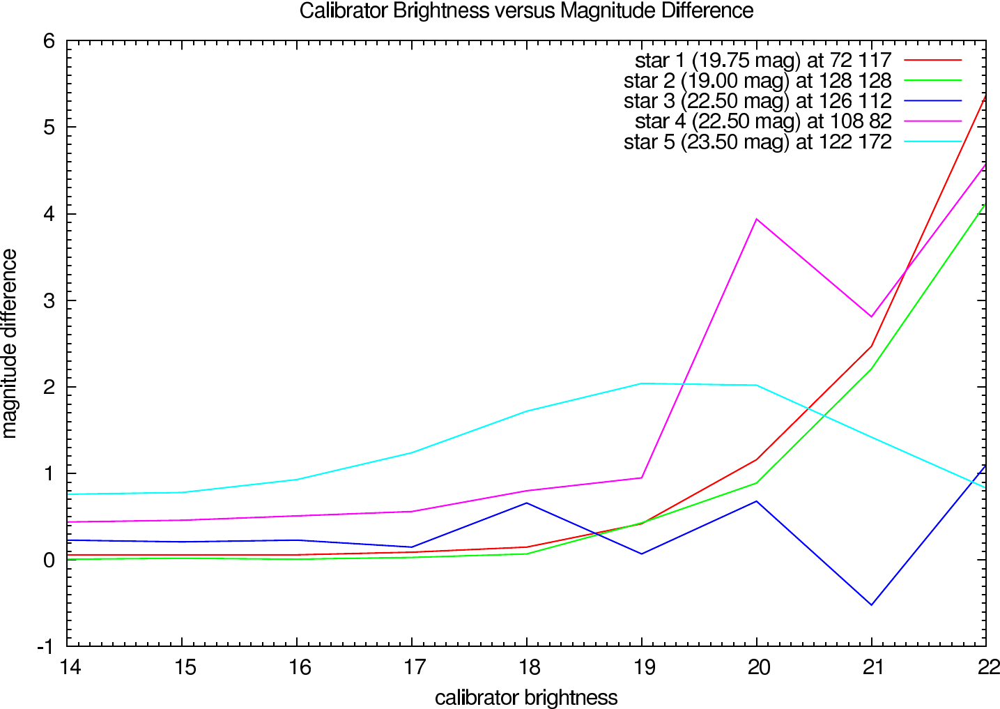
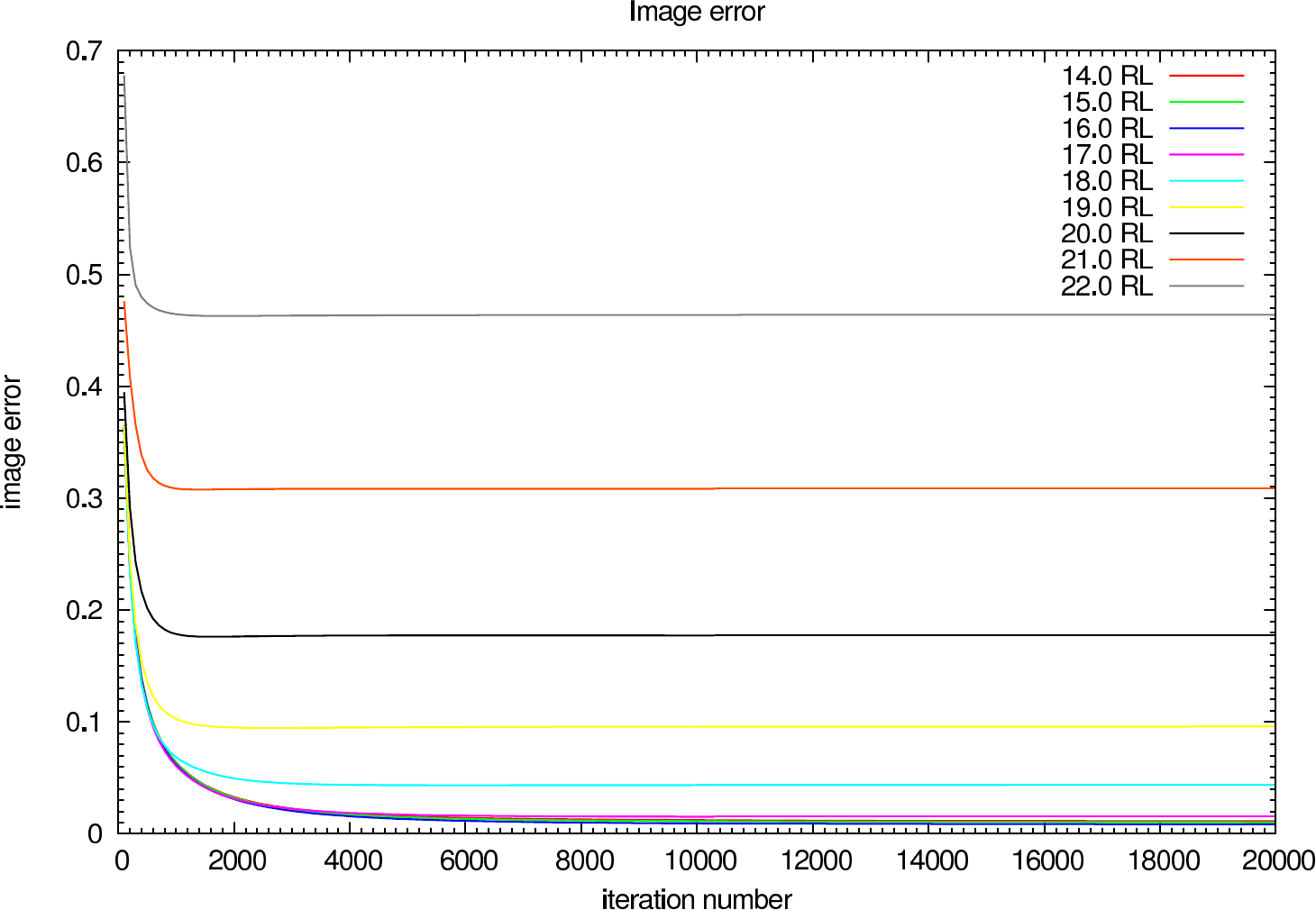
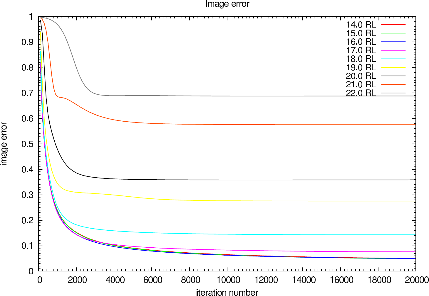
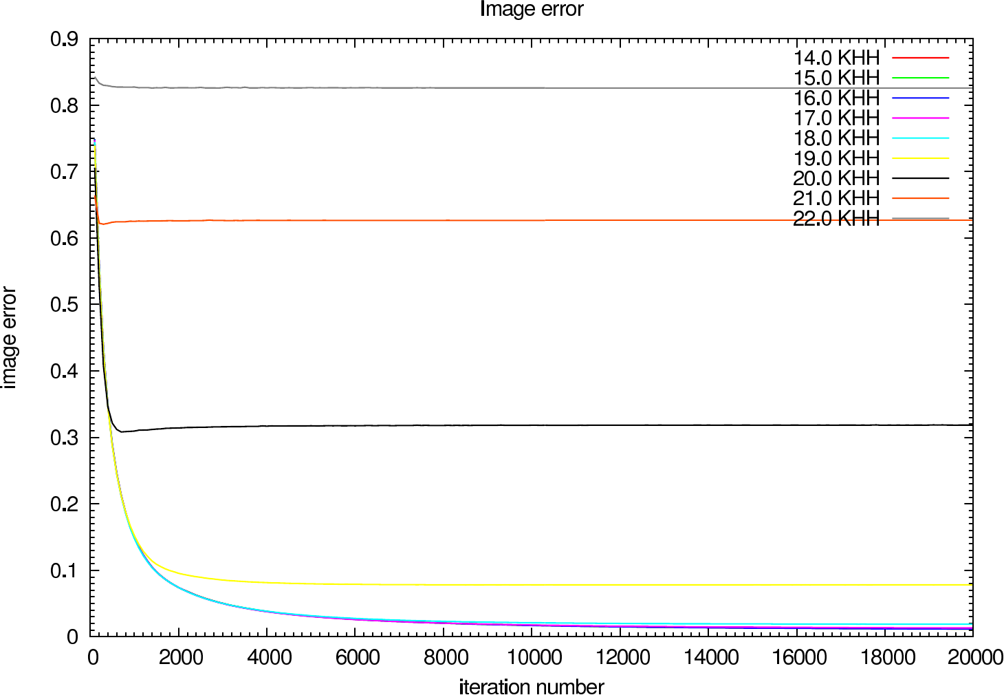
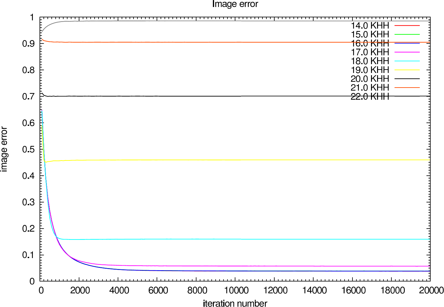
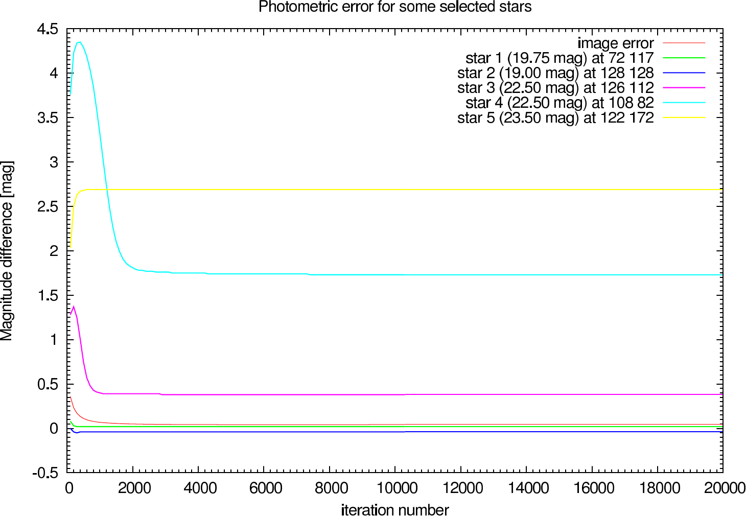
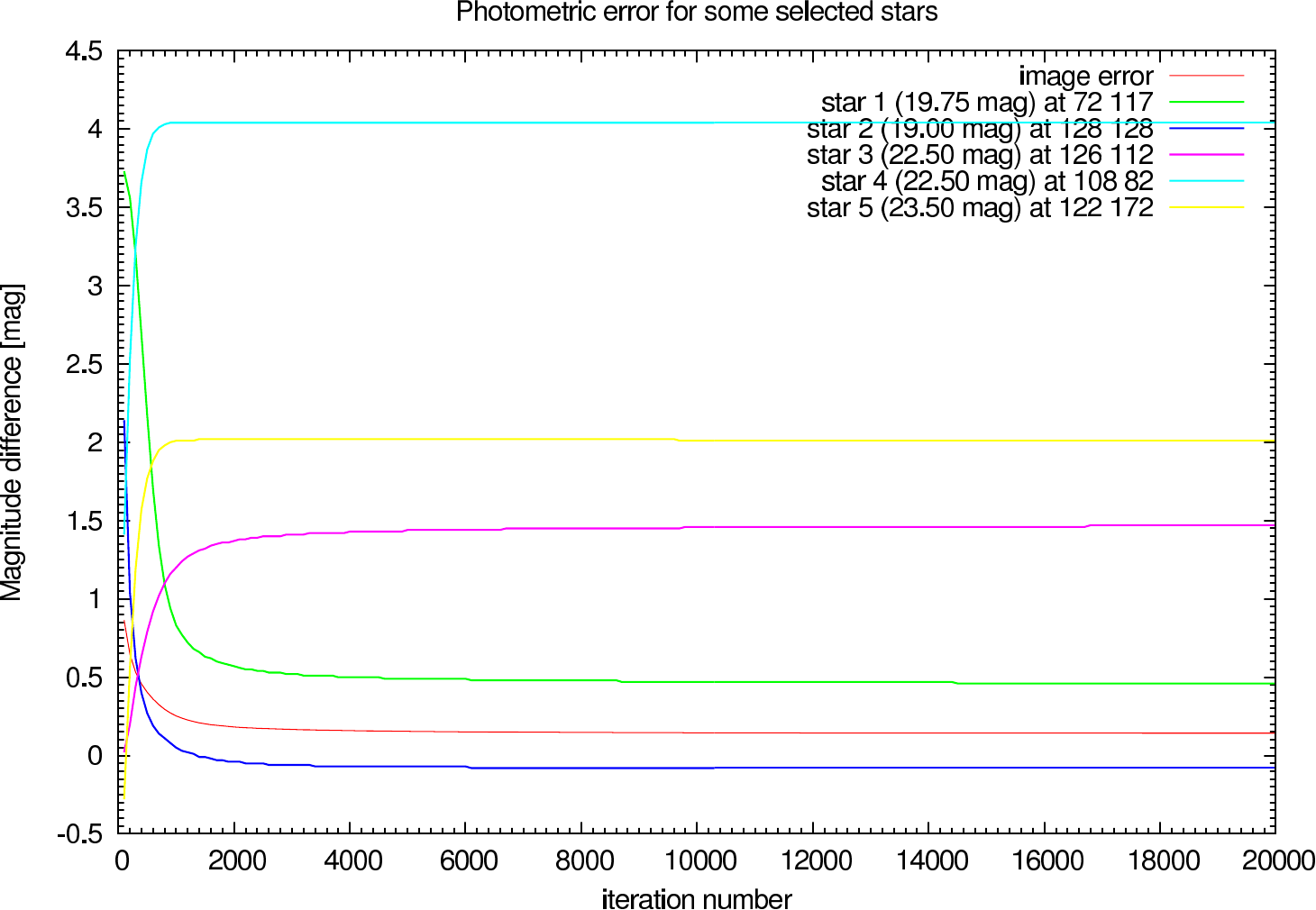
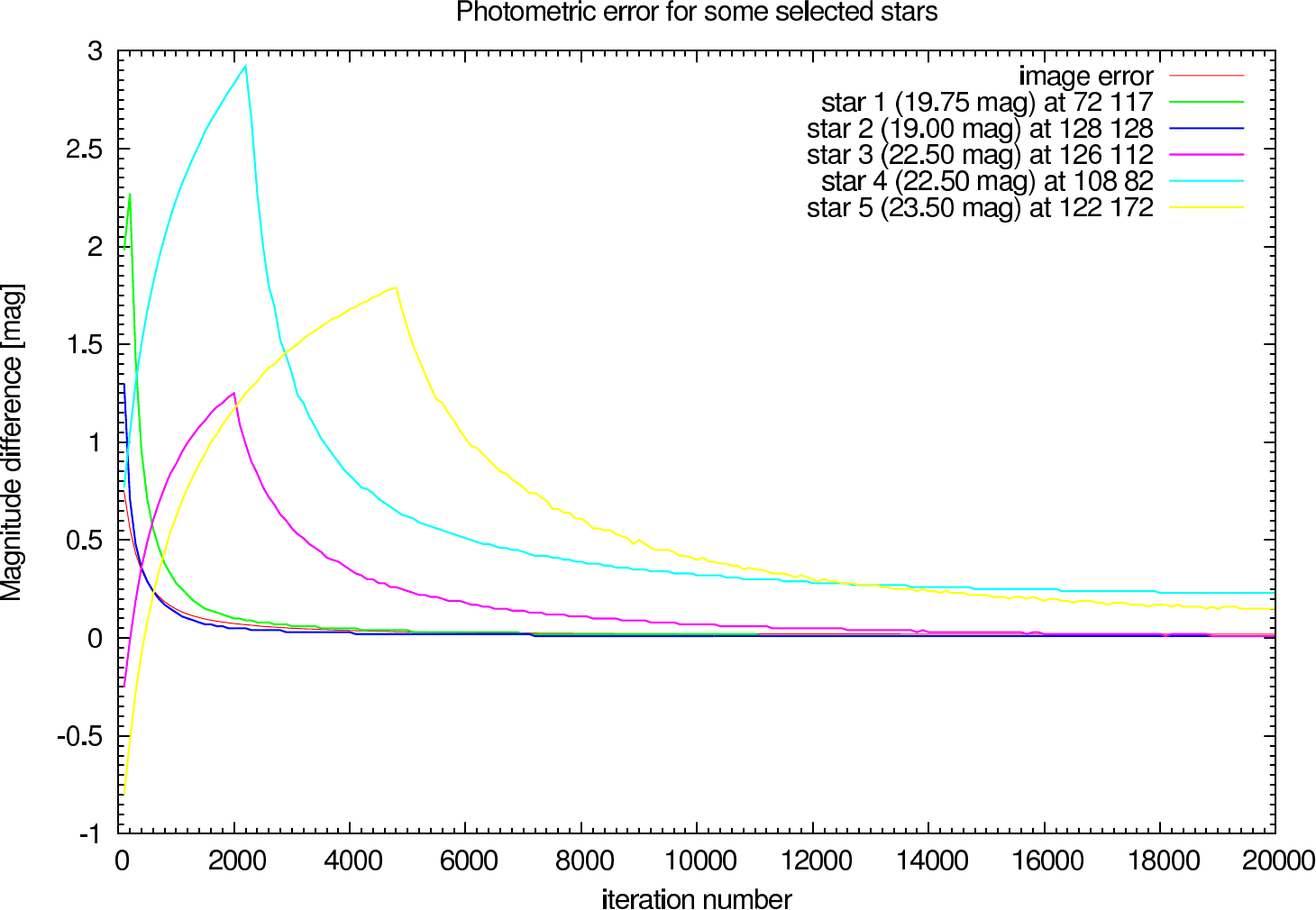
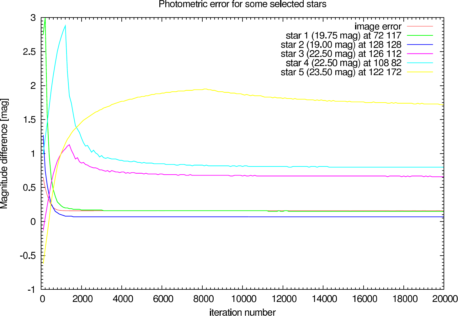
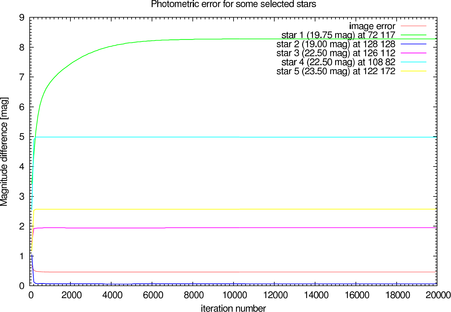
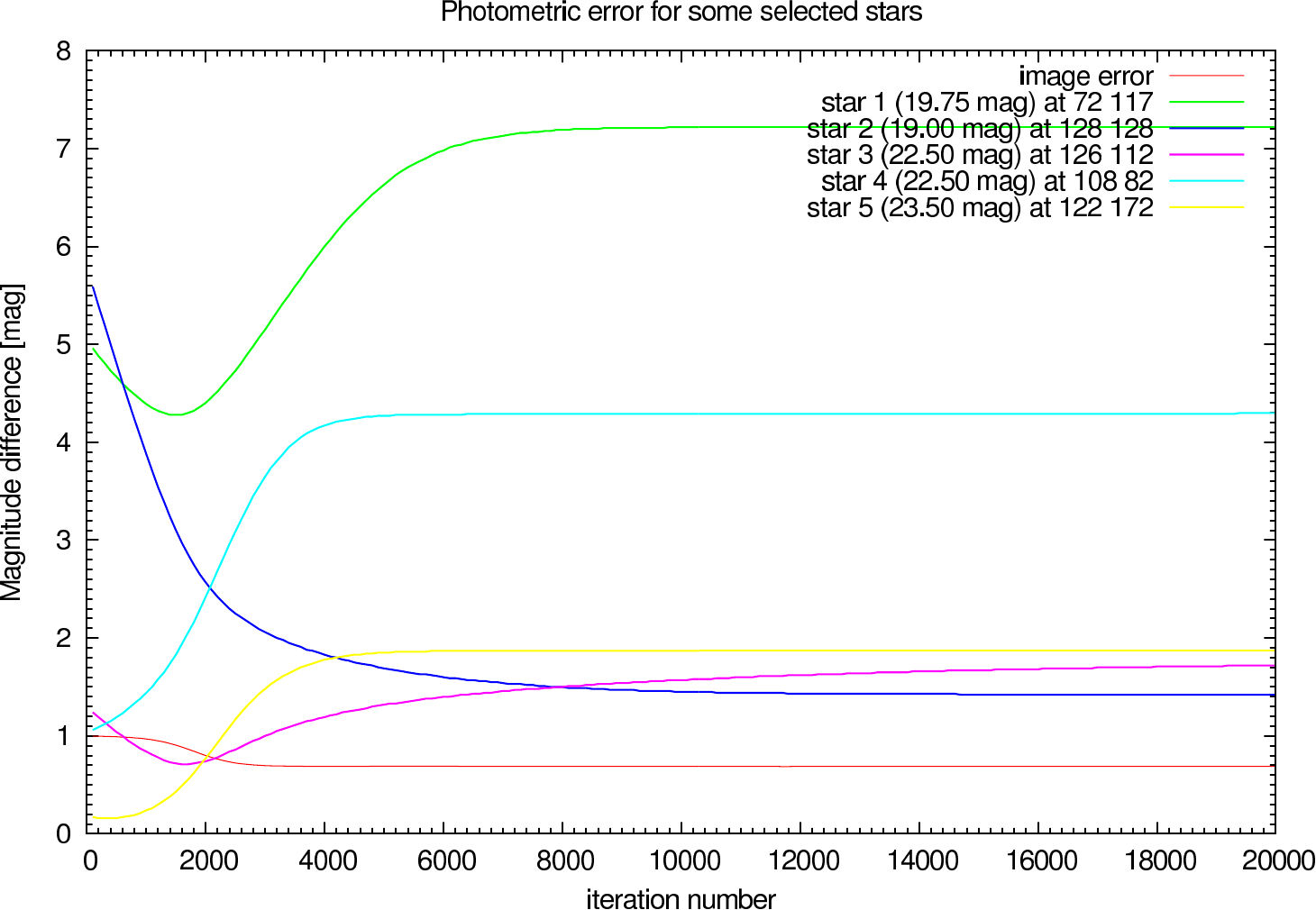
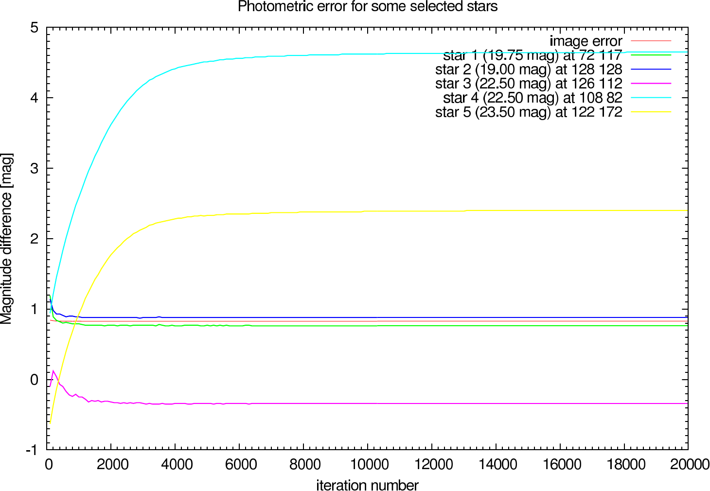
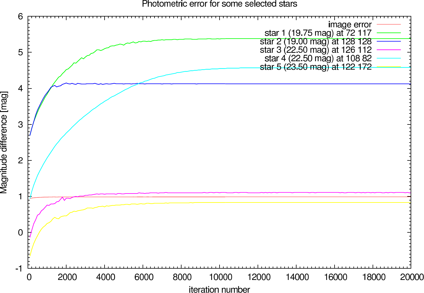
In table 4 (J-Band) and table 5 (K-Band) the errors for the star cluster depending on the psf star brightness are presented. The image errors are also summarized in figure 13 and the photometric errors in figure 14.

Figure 13: In this figure, the image errors depending on the calibrator brightness are shown.

Figure 14: Photometric errors depending on the calibrator bightness in the J-Band (left side) and K-Band (right side). The reconstruction in the first row uses the Richardson-Lucy algorithm, in the second row, the Building-Block method was used.

In figure 15 the image error describing the difference between the reconstruction and the reference image is shown for each iteration (in steps of 100 iterations). The effect of the calibratior brightness on the reconstruction error and the optimal iteration number is clearly visible.

Figure 15: Reconstruction error depending on the iteration number for the J-Band (left side) and the K-Band (right side). The reconstruction in the first row uses the Richardson-Lucy algorithm, in the second row, the Building-Block method was used.

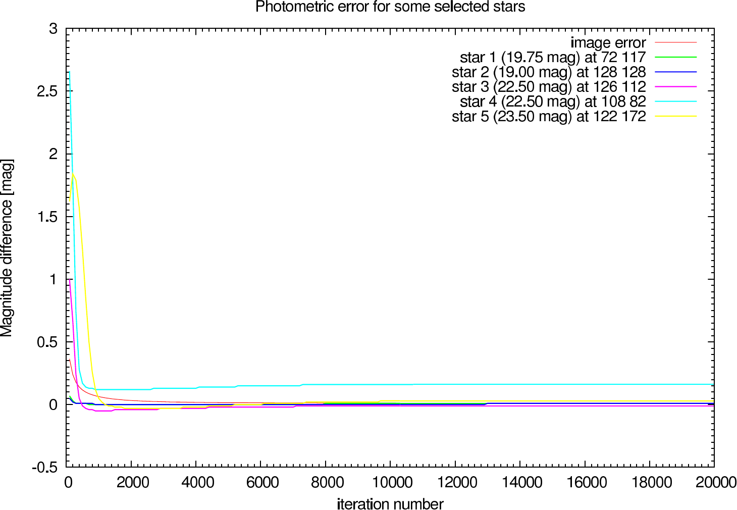
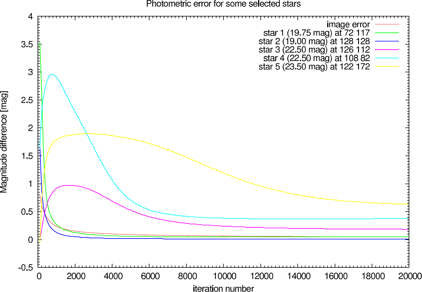
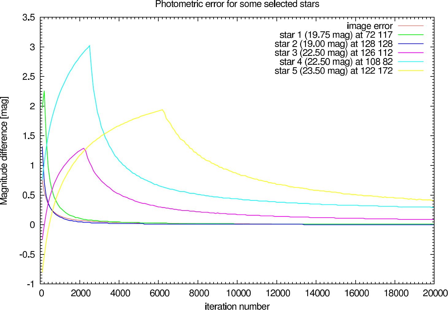
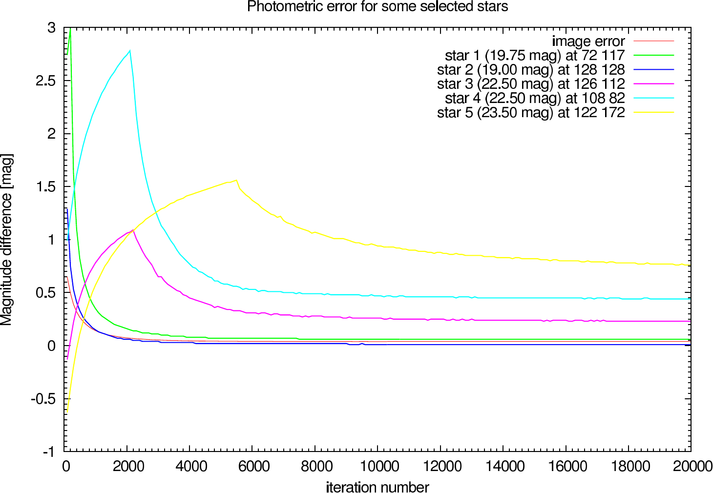
In figure 16, figure 17, and figure 18 the image and photometric errors depending on the calibrator brightness and the iteration number is shown. The overall shape is the same, but the optimum number of iterations is difficult to select, because not all photometric errors have their minimum at the same iteration number.

Figure 16: Image and photometric errors depending on the iteration number in the J-Band (left side) and K-Band (right side). The calibrator brightness is 14 mag. The reconstruction in the first row uses the Richardson-Lucy algorithm, in the second row, the Building-Block method was used.

Figure 17: Image and photometric errors depending on the iteration number in the J-Band (left side) and K-Band (right side). The calibrator brightness is 18 mag. The reconstruction in the first row uses the Richardson-Lucy algorithm, in the second row, the Building-Block method was used.

Figure 18: Image and photometric errors depending on the iteration number in the J-Band (left side) and K-Band (right side). The calibrator brightness is 22 mag. The reconstruction in the first row uses the Richardson-Lucy algorithm, in the second row, the Building-Block method was used.