This simulation investigates the influence of the FFTS performance on the quality of the reconstructions. This means that the AO will give a strehl of 0.30 and the FFTS will give a residual OPD error.

The setup of the simulation is described in table 1. The input data for the test uses a strehl value of 0.30 for the target and the calibrator which has a magnitude of 14. In addition the target and calibrator images are influenced by a gaussian distributed phase error with the same standard deviation, resulting in a fringe contrast loss. This error is modelled as a phase error on the second pupil and for each phase screen (the properties of the atmosphere will result in about 600 phase screens per position angle) a random phase error is introduced. This phase error is specified as a gaussian error with a standard deviation of the OPD between 0.0 (perfect FFTS) and 0.5 lambda (worst case, no FFTS available).

The raw data were generated according to the common scheme described in section Overview. In addition the phase screens for the psfs are influenced by a phase error on the second pupil, and the images for the target and psf-star are generated separately which means, that the calibrator image is not influenced by the target (no halo, etc.).

All simulated input data for the LN DRS pipeline are available as a tar-file (ex3_j_input.tar.gz (18MB) and ex3_k_input.tar.gz (20MB)). The corresponding results are also available as tar files (ex3_j_results.tar.gz (2.7MB) and ex3_k_results.tar.gz (2.8MB)).

The generated calibrator raw images are shown in section Calibrator. The raw images and deconvolution results are shown in section Raw Frames and Results for an AGN for the AGN and section Raw Frames and Results for a Star Cluster for the star cluster.

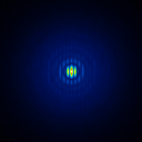
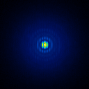
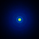
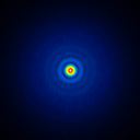
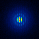
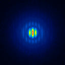
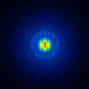
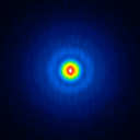
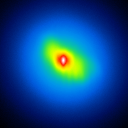
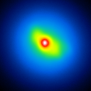
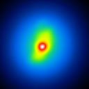
The simulated raw LBT interferograms used for the deconvolution are ideal images, they are not influenced by detector effects like different pixel gain or bad pixels. In figure 1 the calibrators for the different phase errors and one position angle are shown.

Figure 1: Central 128x128 pixels of the generated J-Band (top row) and K-Band (bottpon row) images of a calibrator with phase errors of (from top left to bottom right) 0.0, 0.1, 0.2, and 0.5 lambda.

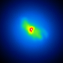
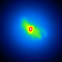
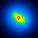
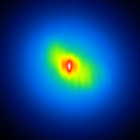
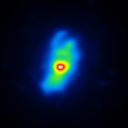
The basis of the simulation is an image of NGC4151 with an overlayed dust torus (see figure 1). The simulated raw images for a position angle of 108 degree are shown in figure 2.

Figure 2: The simulated J-Band (top row) and K-Band (bottom row) raw images for a position angle of 108 degree of NGC4151 at 10.1 mag including sky background with a phase error of 0.0, 0.1, 0.2, and 0.5 lambda (from left to right).

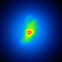
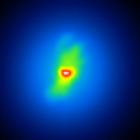
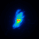
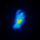
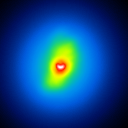
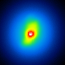
A comparison of the reconstructions depending on the phase error is presented in figure 3 for the J-Band. For the K-Band the results are presented in figure 4.

Figure 3: The top row shows the coadded J-Band raw images. The second row show the reconstructions using the Richardson-Lucy algorithm. The phase error is 0.0, 0.1, 0.2, and 0.5 lambda (from left to right). In the third row, the Building-Block algorithm was used

Figure 4: The top row shows the coadded K-Band raw images. The second row show the reconstructions using the Richardson-Lucy algorithm. The phase error is 0.0, 0.1, 0.2, and 0.5 lambda (from left to right). In the third row, the Building-Block algorithm was used.

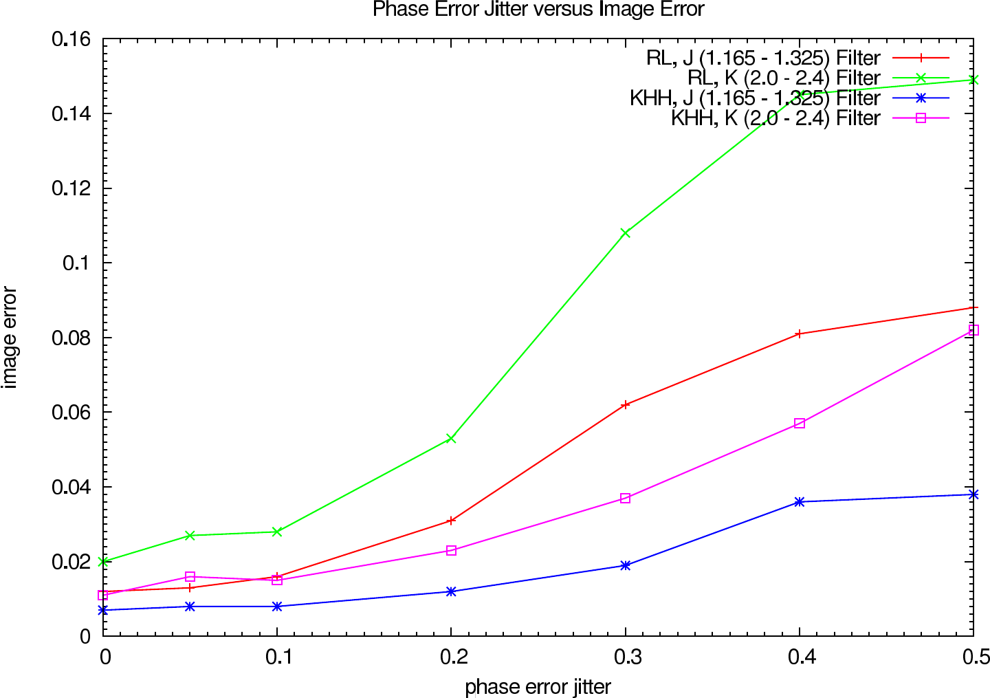
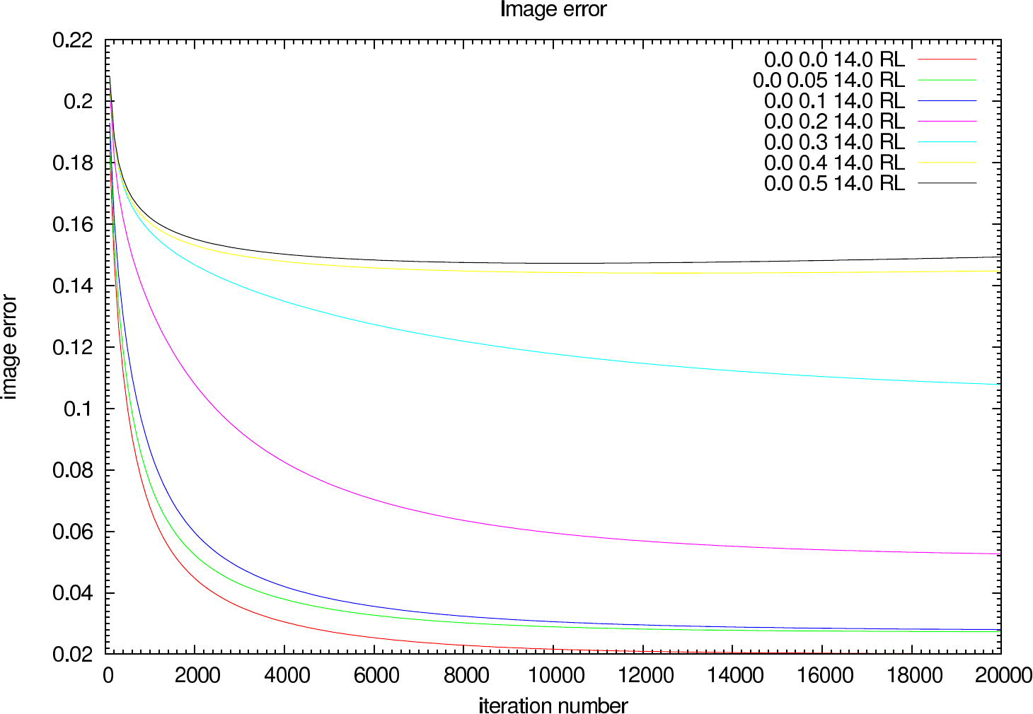
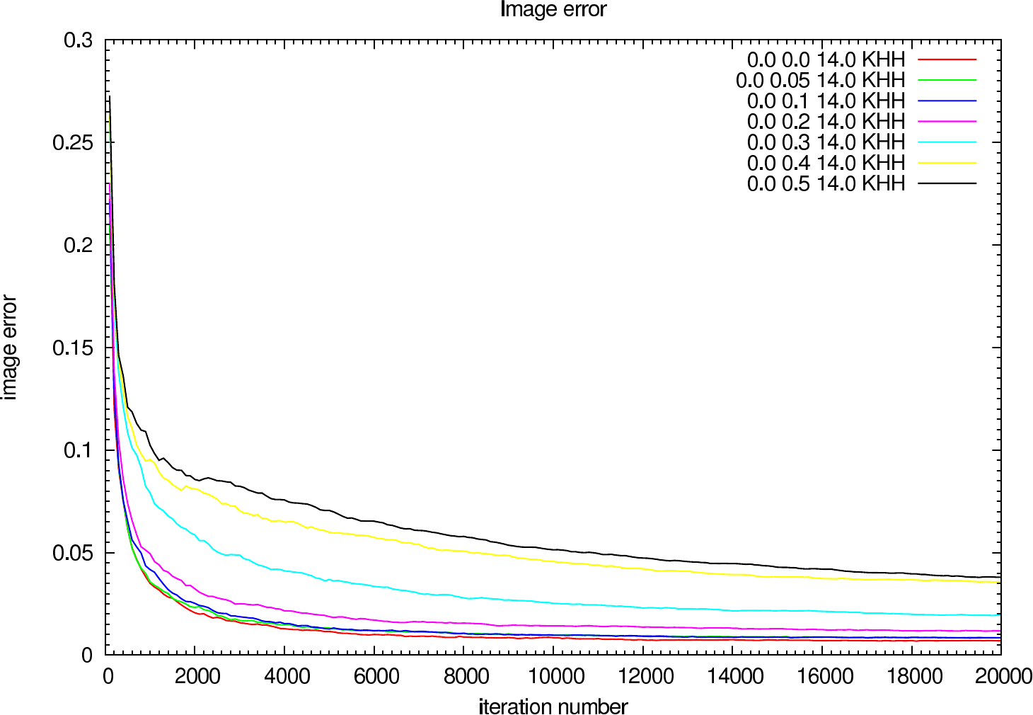
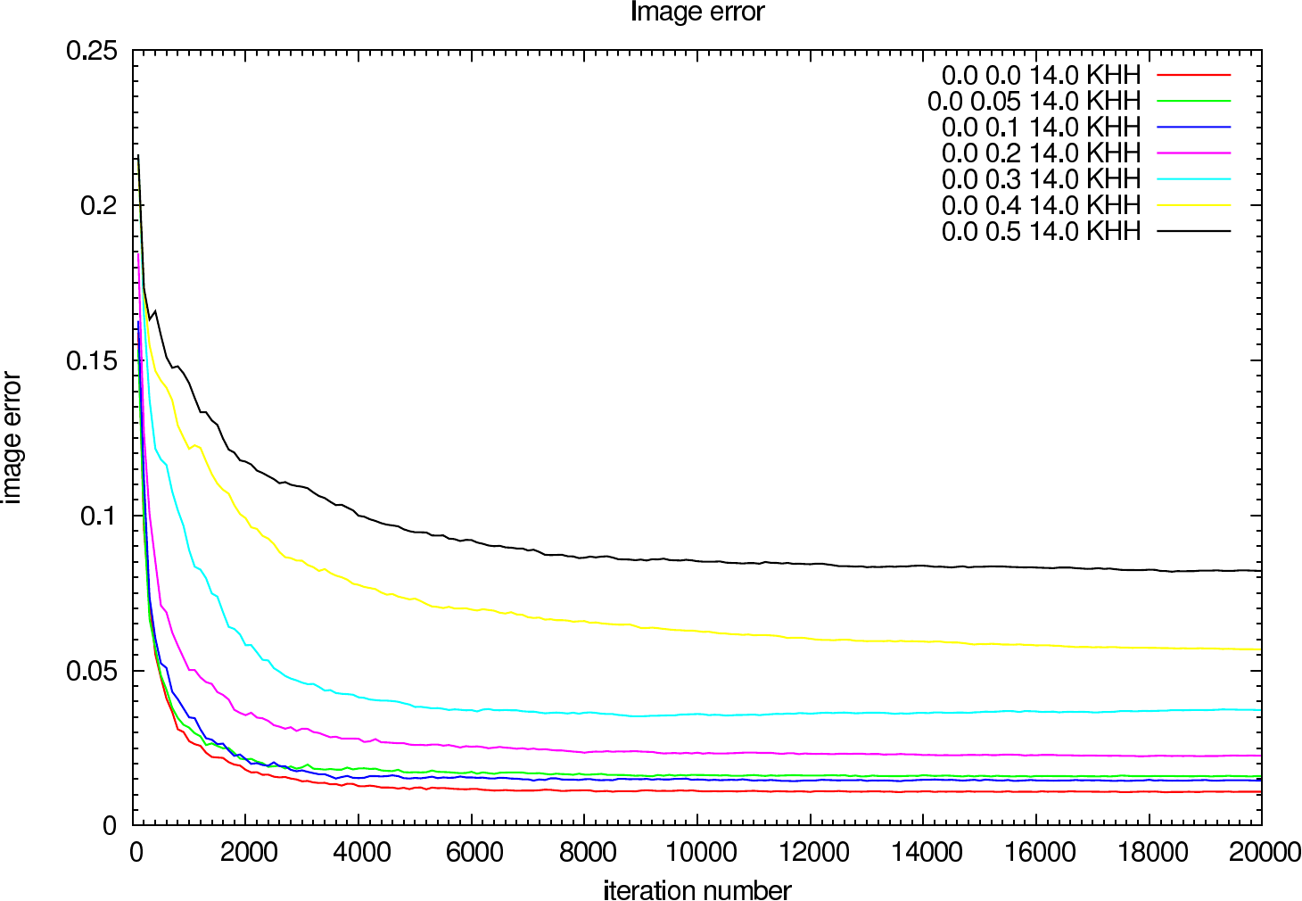
In table 2 (J-Band) and table 3 (K-Band) the errors for the star cluster depending on the OPD error are presented. In figure 5 the image errors depending on the phase error jitter are shown.

Figure 5: In this figure, the image errors depending on the phase error jitter are shown.

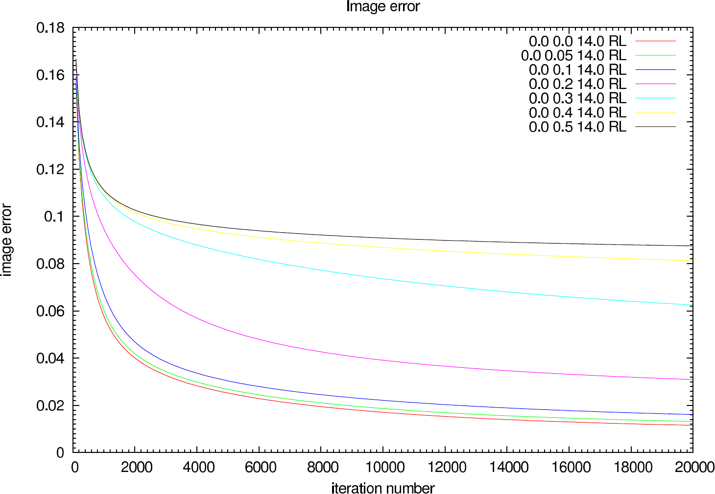
In figure 6 the image error describing the difference between the reconstruction and the reference image is shown for each iteration (in steps of 100 iterations). The effect of the OPD error on the reconstruction error and the optimal iteration number is clearly visible.

Figure 6: Reconstruction error depending on the iteration number for the J-Band (left side) and K-Band (right side). For the reconstructions in the top row, Richardson-Lucy was used. In the second row, the Building-Block algorithm was used.

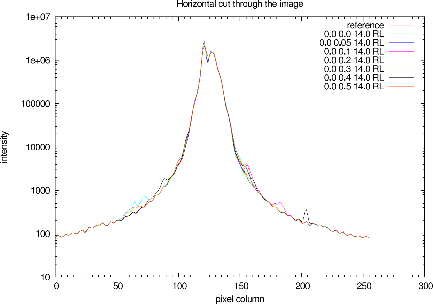
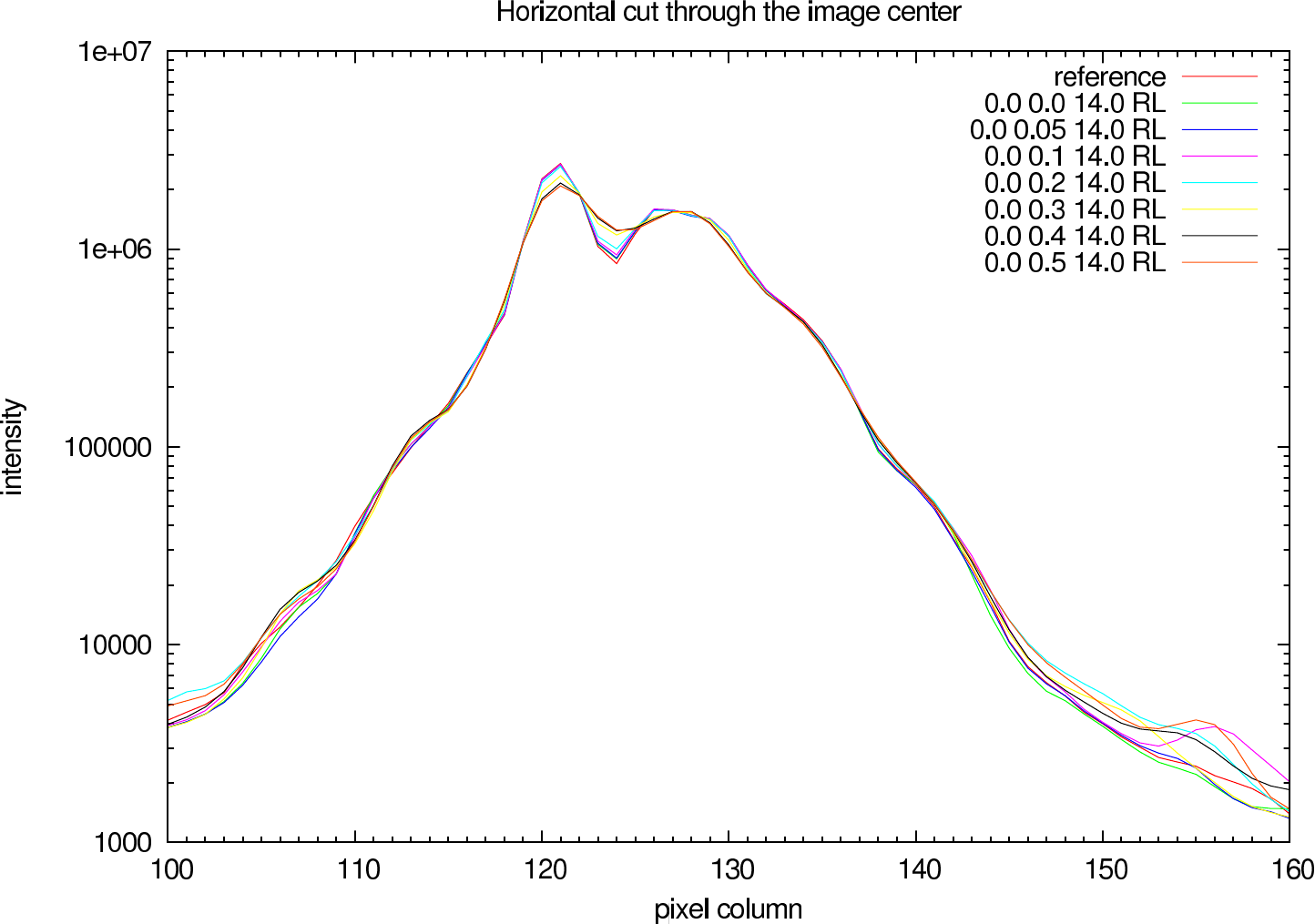
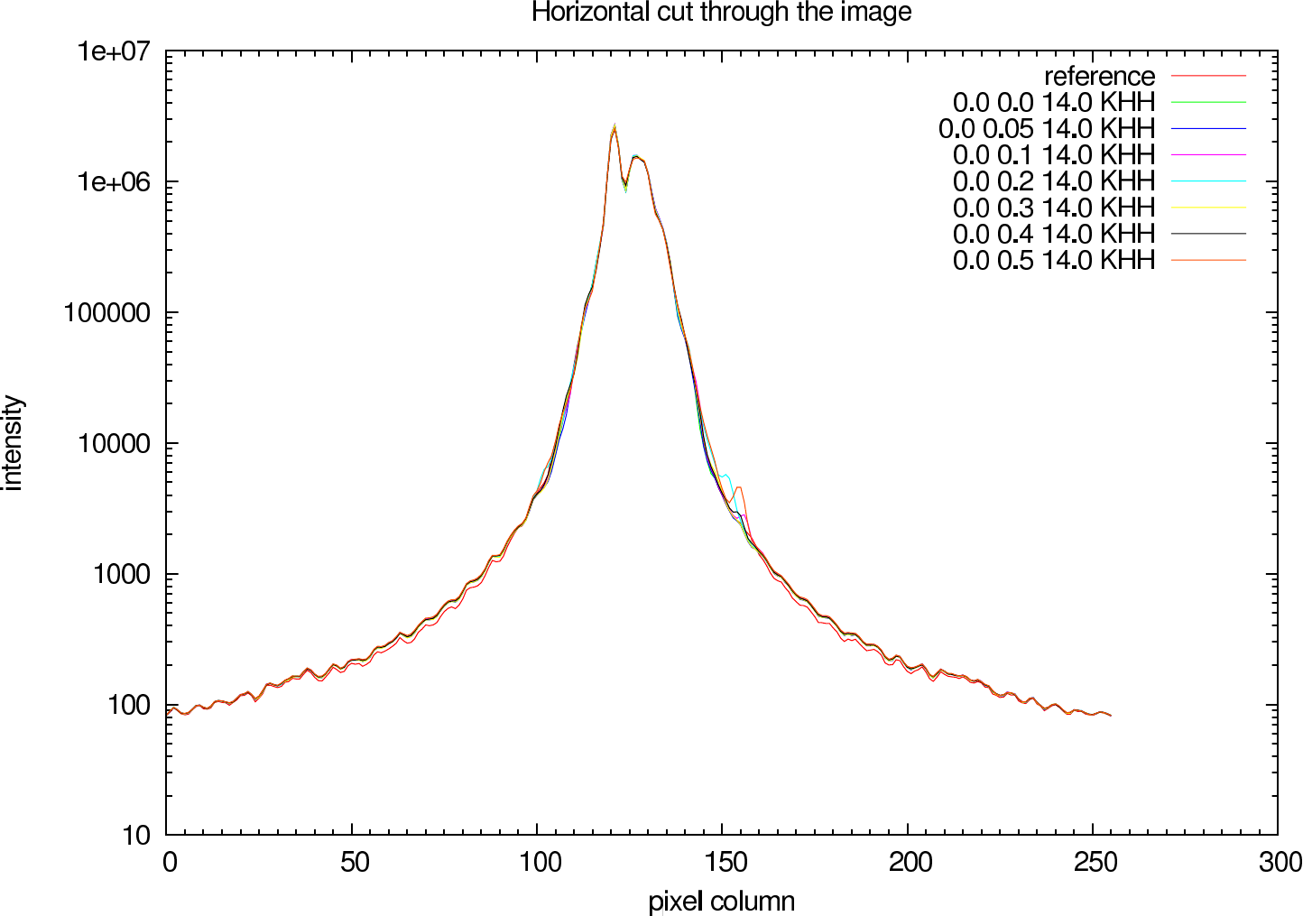
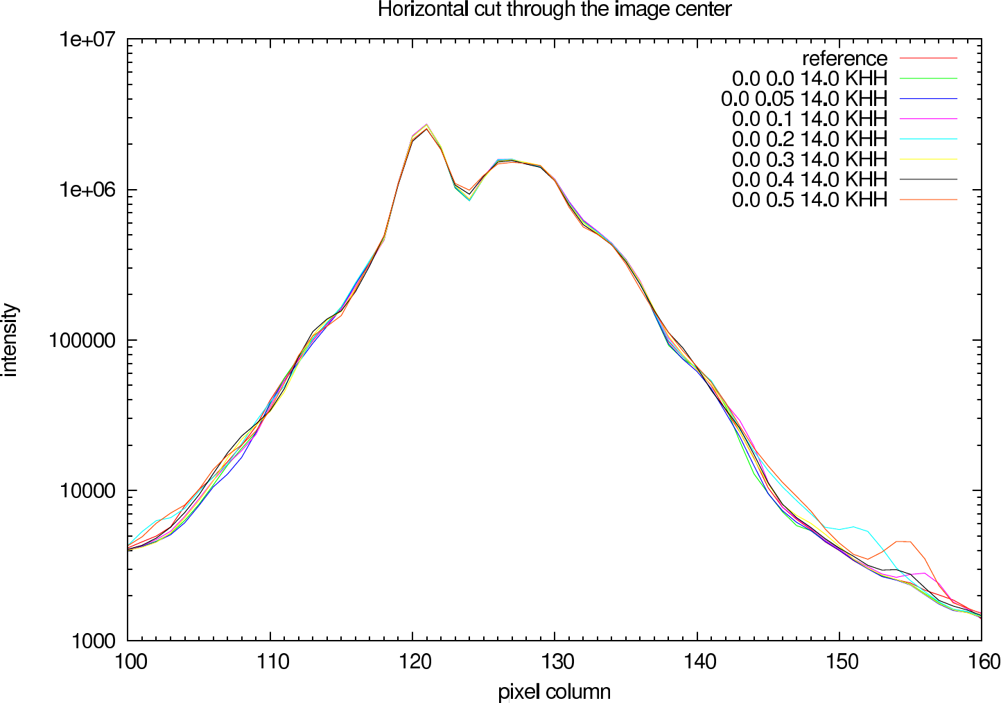
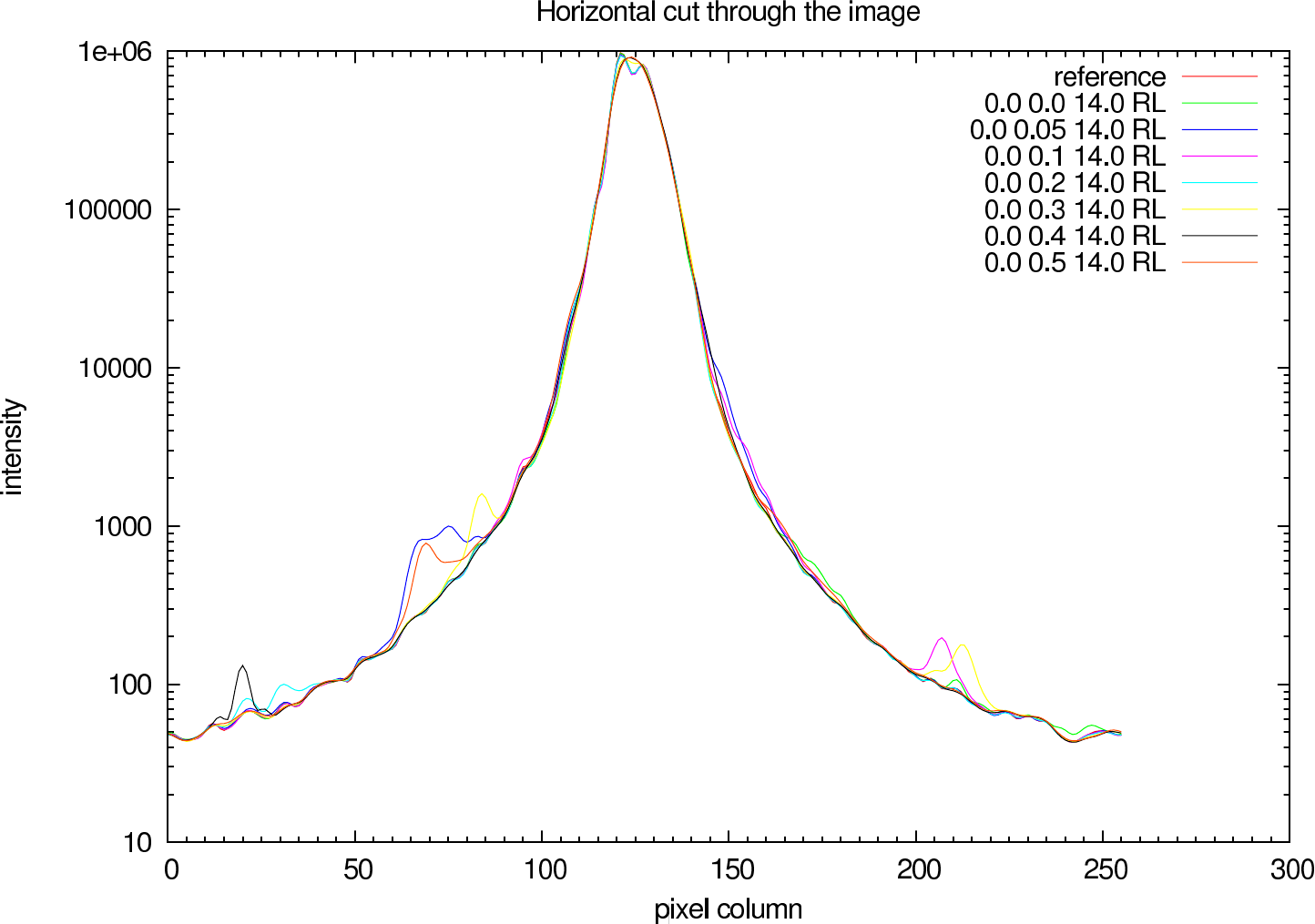
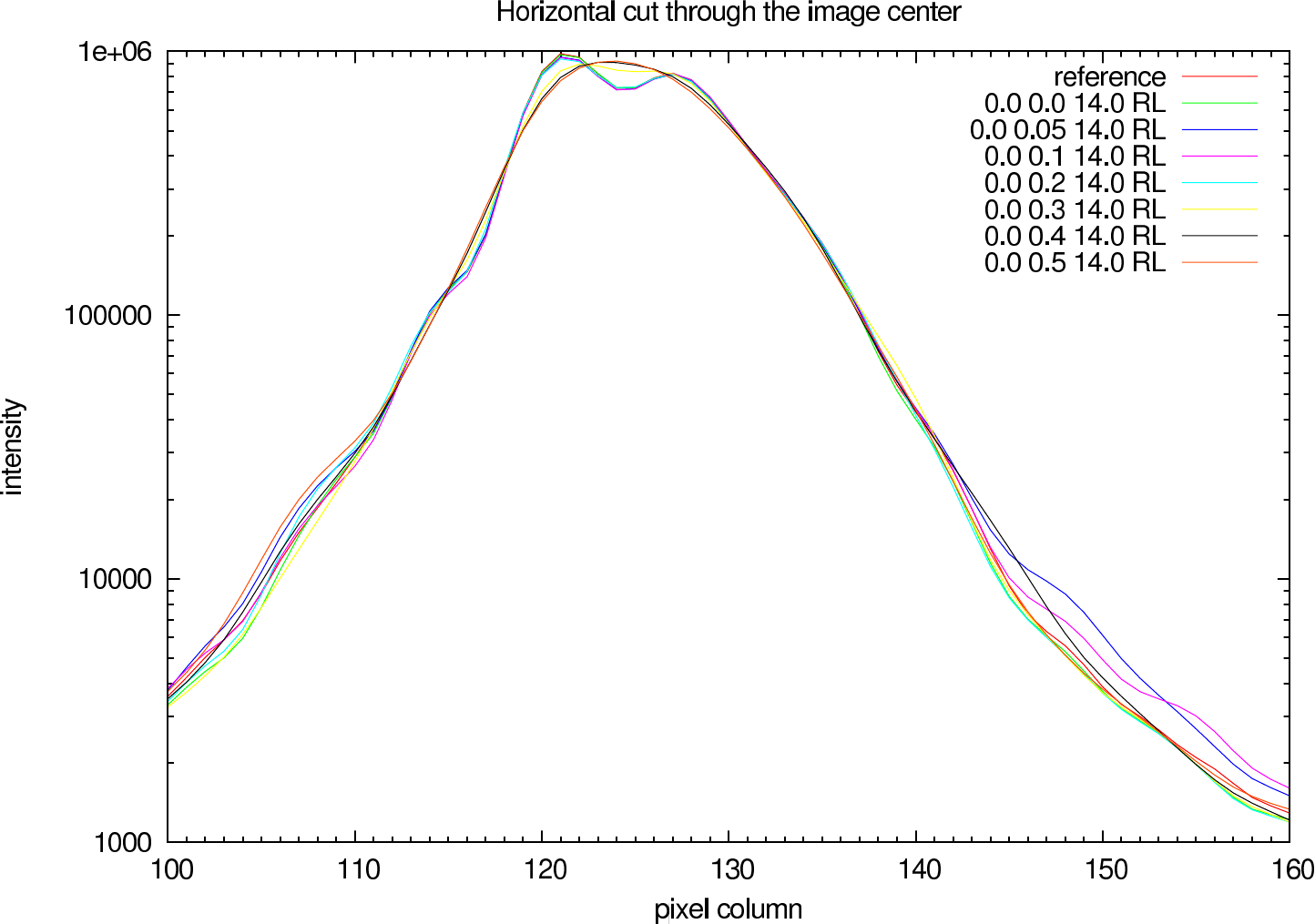
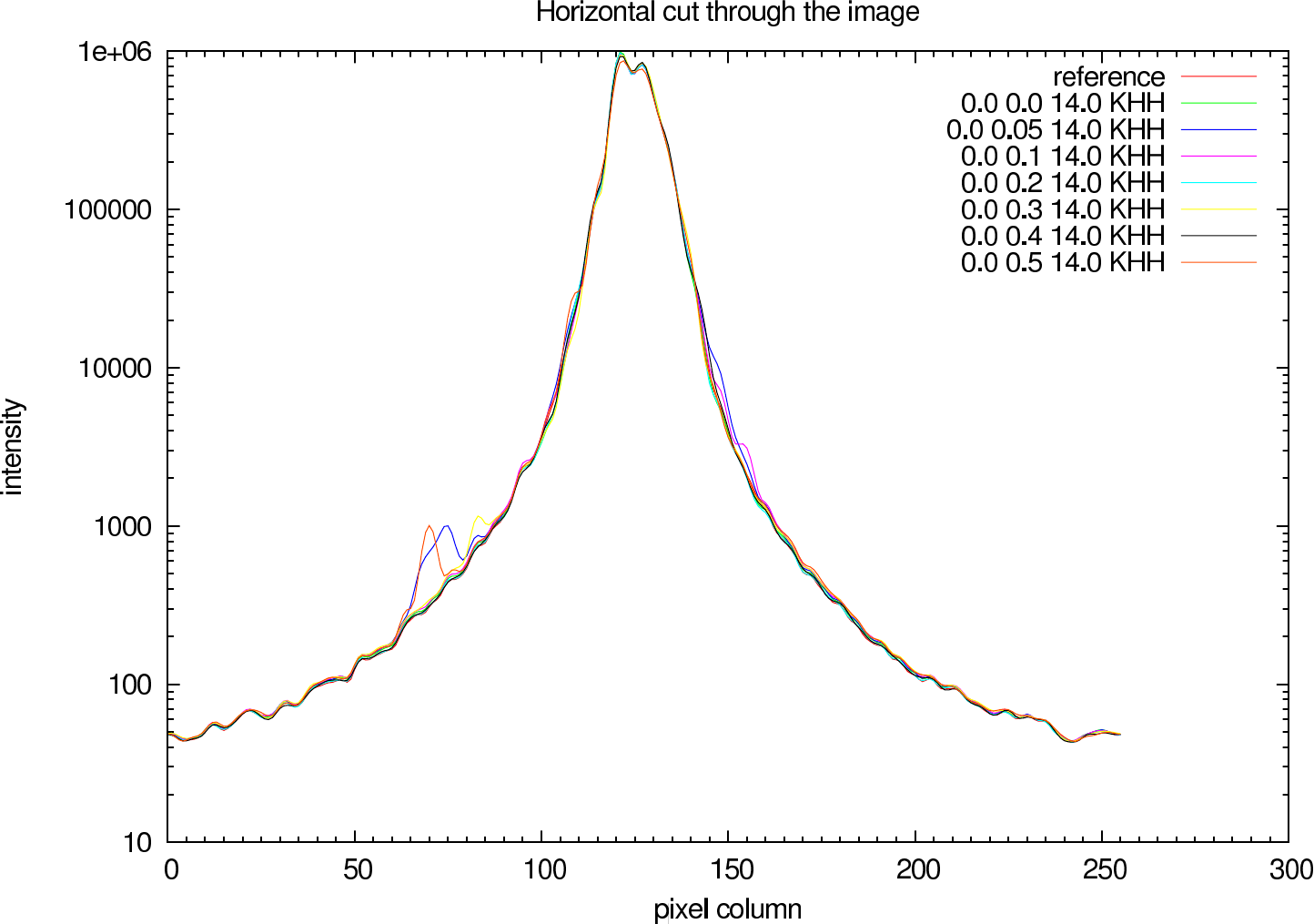
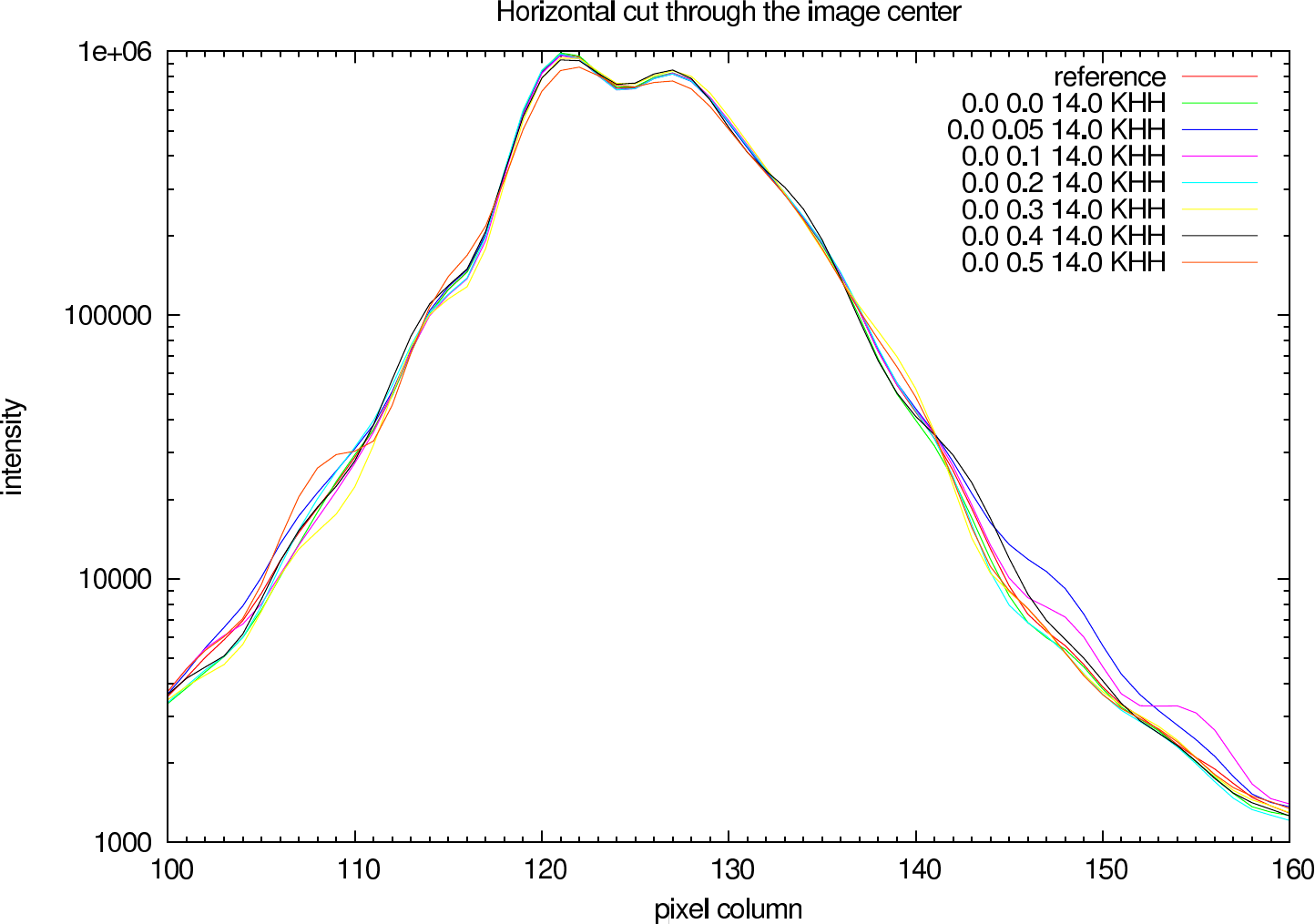
In figure 7 (J-Band) and figure 8 (K-Band) a horizontal cut slightly above the intensity maximum of the reconstructions of NHC4151 compared with the ideal reference image is shown.

Figure 7: Horizontal profile through the center of the reconstructed galaxy compared to the ideal image (J-Band). On the right side only the central part is shown. For the reconstructions in the top row, Richardson-Lucy was used. In the second row, the Building-Block algorithm was used.

Figure 8: Horizontal profile through the center of the reconstructed galaxy compared to the ideal image (K-Band). On the right side only the central part is shown. For the reconstructions in the top row, Richardson-Lucy was used. In the second row, the Building-Block algorithm was used.

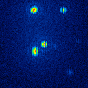
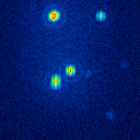
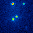
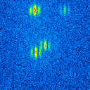
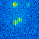
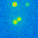
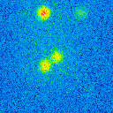
The basis of the simulation is an image of a star cluster (see figure 2). The simulated raw images for a position angle of 108 degree are shown in figure 9.

Figure 9: The simulated J-Band (top row) and K-Band (bottom row) raw images for a position angle of 108 degree of the star cluster at 10.1 mag including sky background with a phase error of 0.0, 0.1, 0.2, and 0.5 lambda (from left to right).

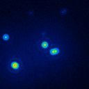
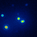
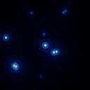
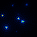
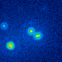
A comparison of the reconstructions depending on the phase error is presented in figure 10 for the J-Band. For the K-Band the results are presented in figure 11.

Figure 10: The top row shows the coadded J-Band raw images. The second row show the reconstructions using the Richardson-Lucy algorithm. The phase error is 0.0, 0.1, 0.2, and 0.5 lambda (from left to right). In the third row, the Building-Block algorithm was used

Figure 11: The top row shows the coadded K-Band raw images. The second row show the reconstructions using the Richardson-Lucy algorithm. The phase error is 0.0, 0.1, 0.2, and 0.5 lambda (from left to right). In the third row, the Building-Block algorithm was used

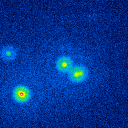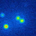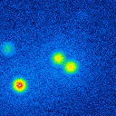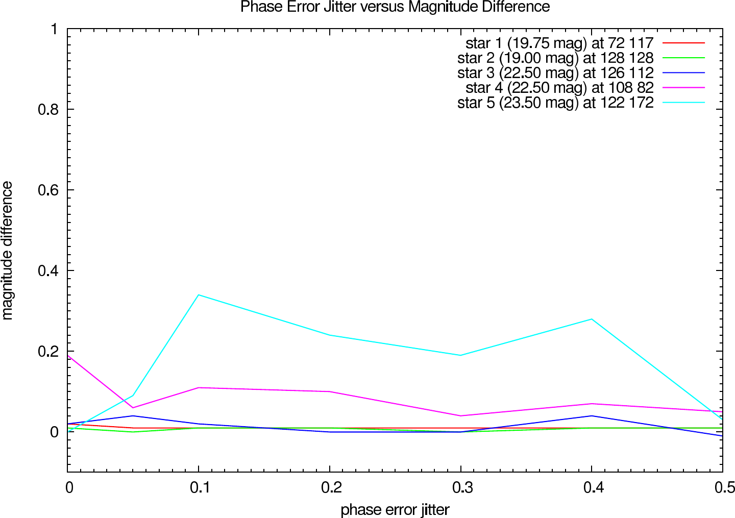
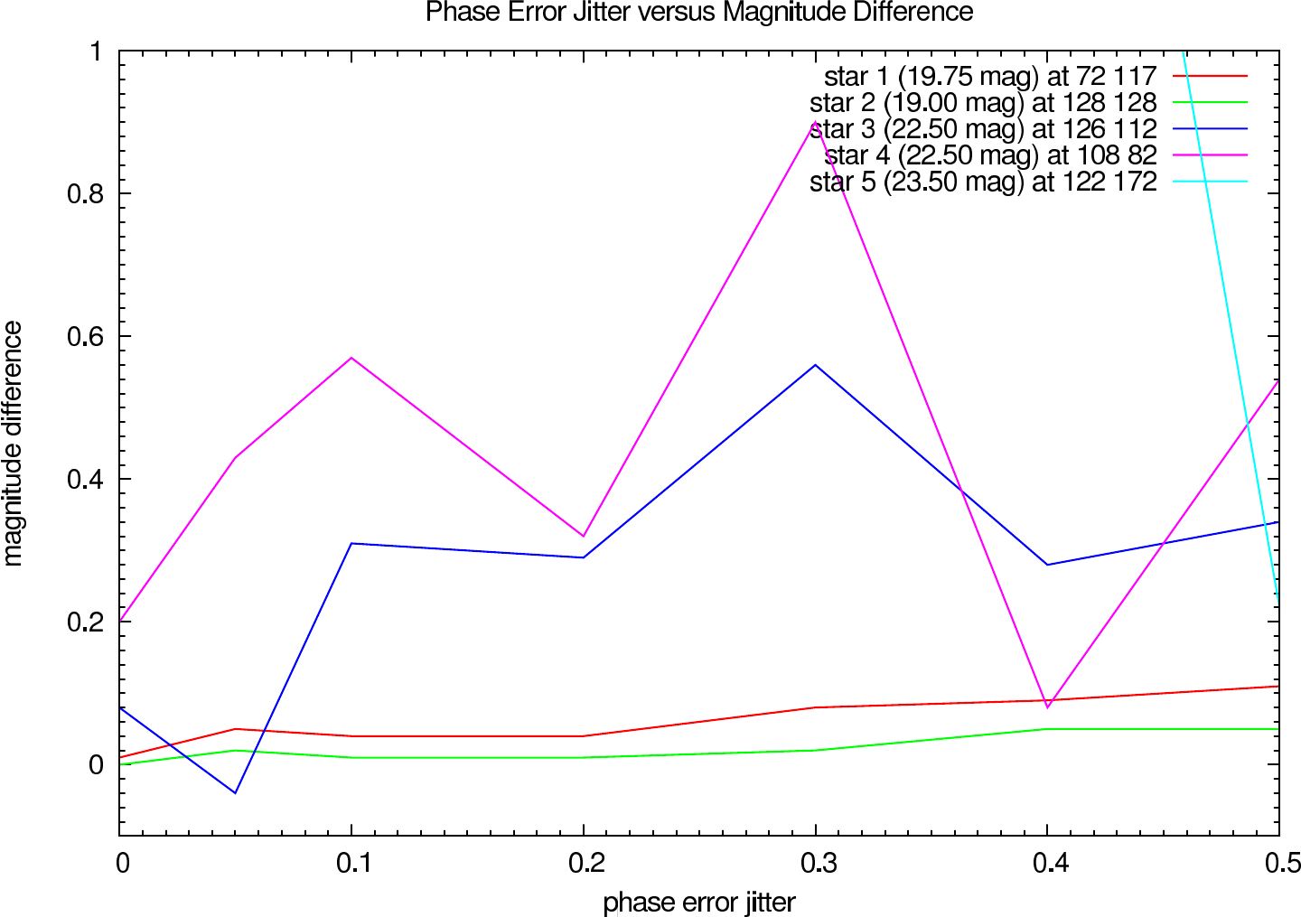
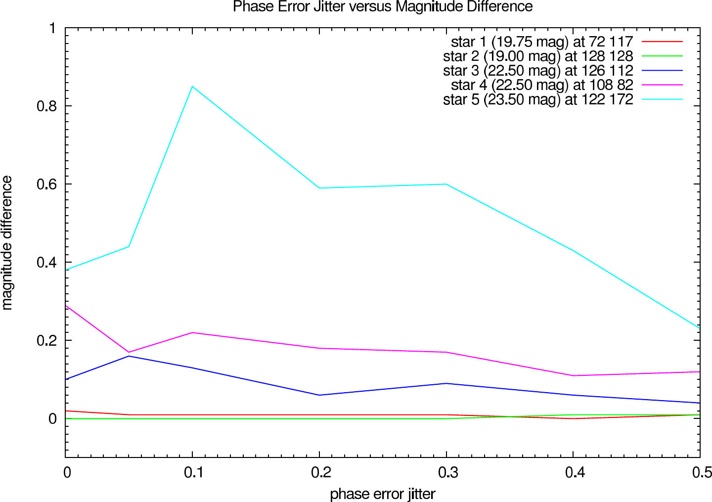
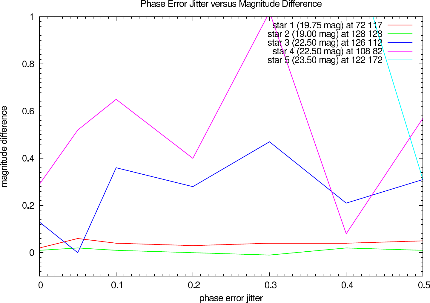
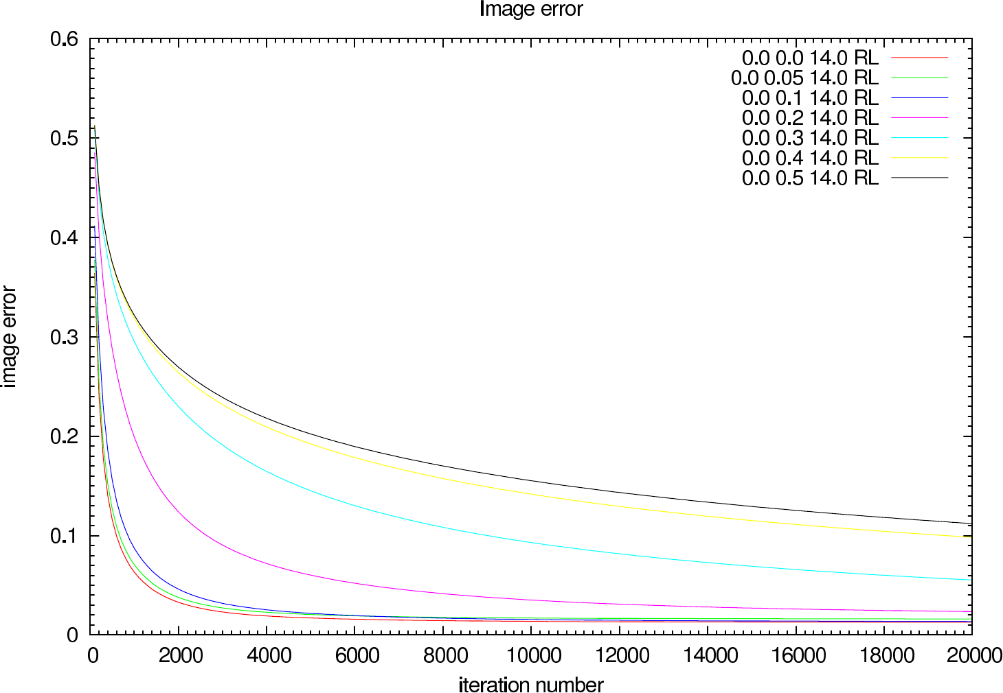
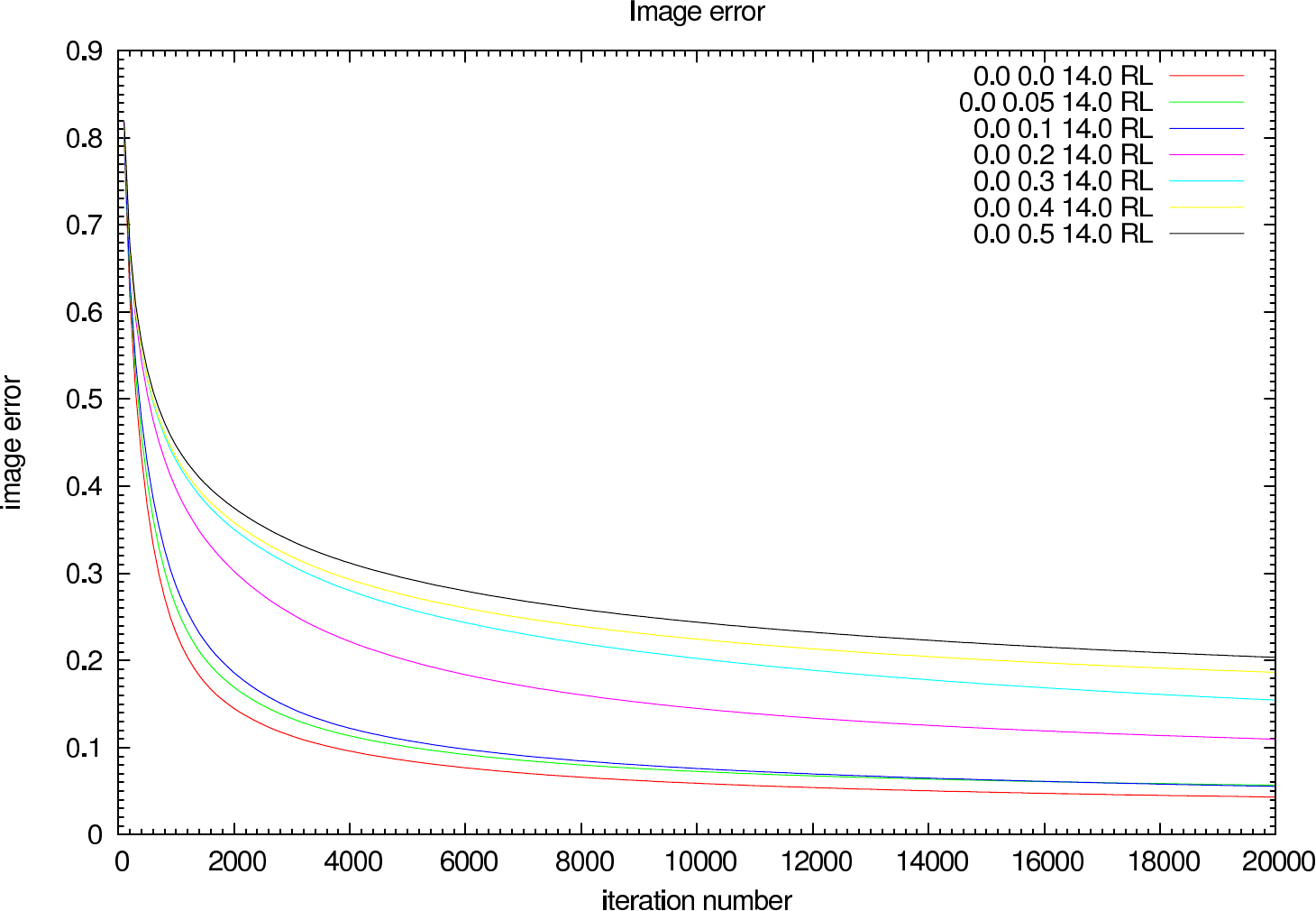
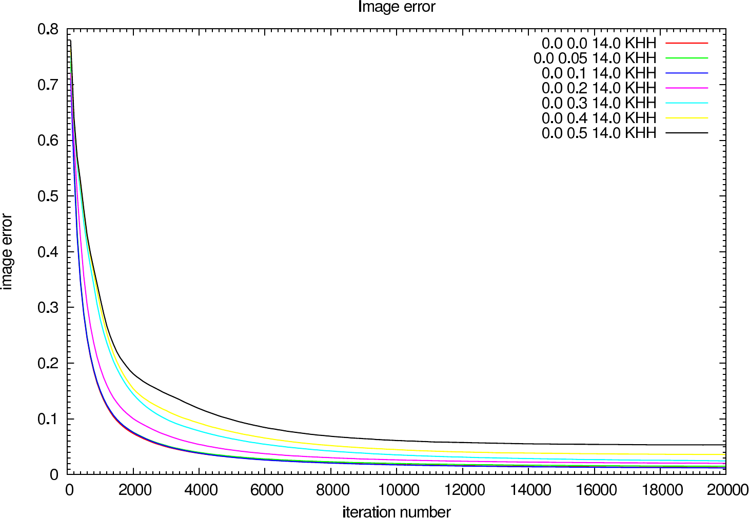
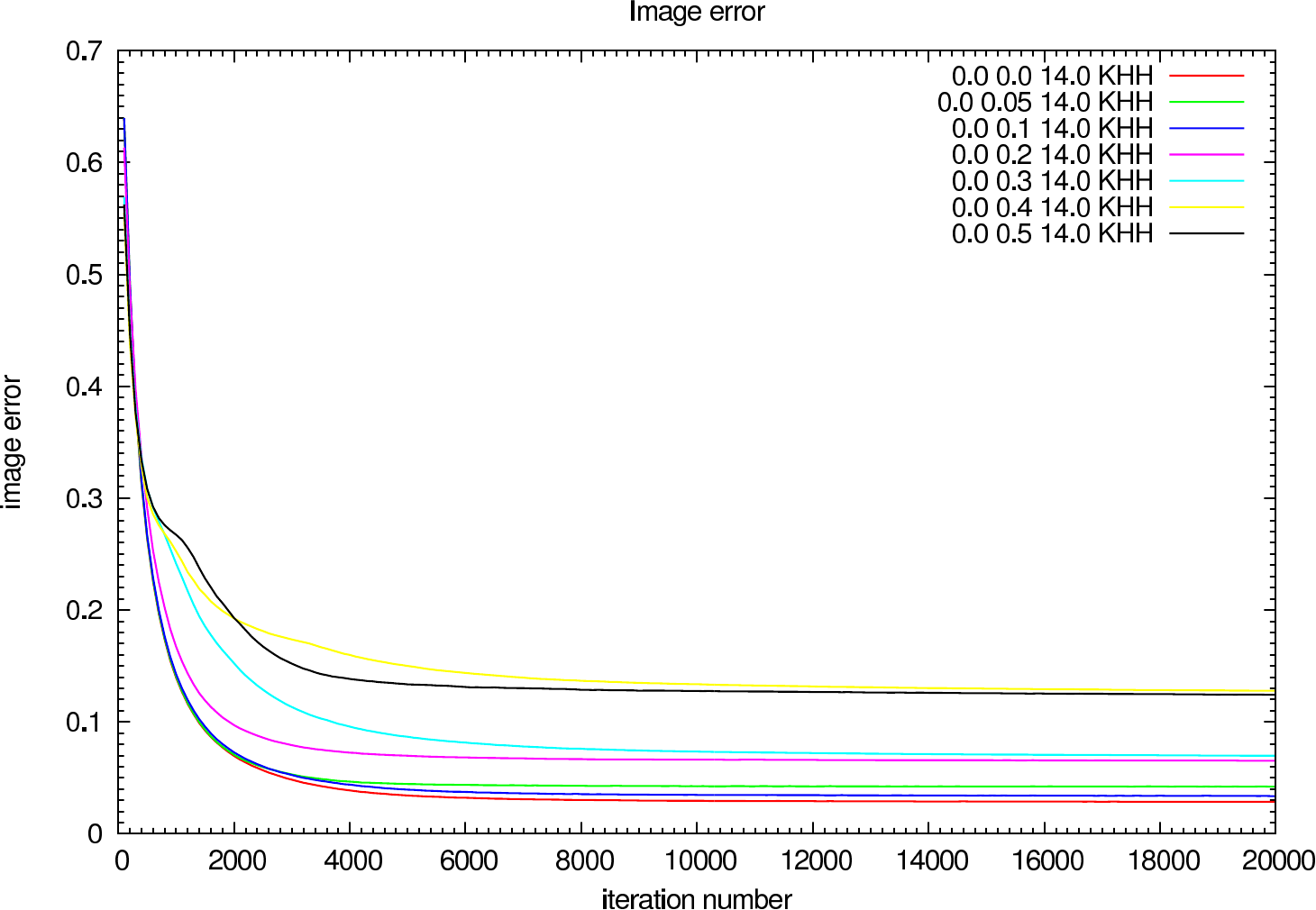
In table 4 (J-Band) and table 5 (K-Band) the errors for the star cluster depending on the OPD error are presented. The image errors are also summarized in figure 12 and the photometric errors in figure 13.

Figure 12: In this figure, the image errors depending on the phase error jitter are shown.

Figure 13: Photometric errors depending on the phase error jitter in the J-Band (left side) and K-Band (right side). The reconstruction in the first row uses the Richardson-Lucy algorithm, in the second row, the Building-Block method was used.

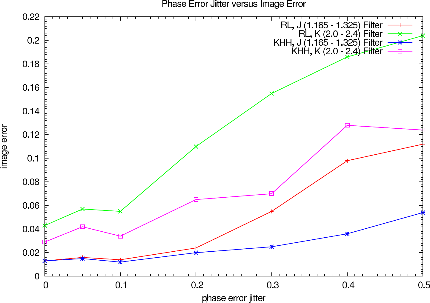In figure 14 the image error describing the difference between the reconstruction and the reference image is shown for each iteration (in steps of 100 iterations). The effect of the OPD error on the reconstruction error and the optimal iteration number is clearly visible.

Figure 14: Reconstruction error depending on the iteration number for the J-Band (left side) and K-Band (right side). For the reconstructions in the top row, Richardson-Lucy was used. In the second row, the Building-Block algorithm was used.

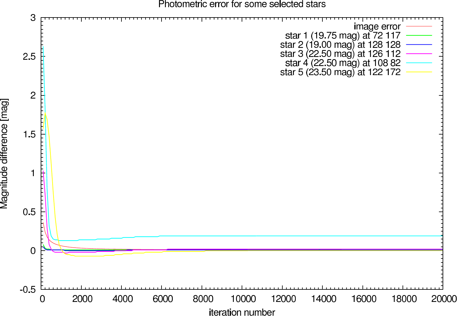
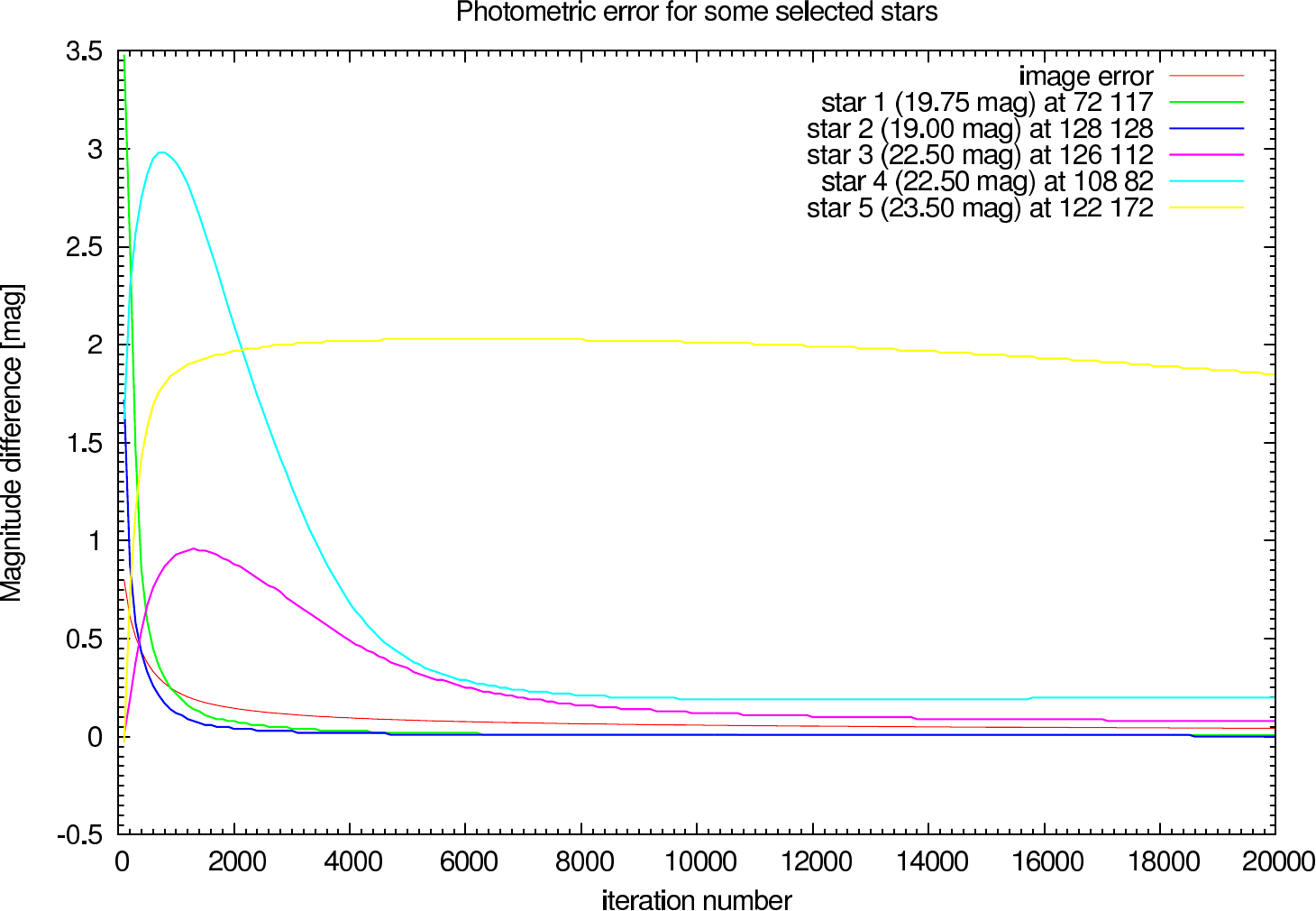
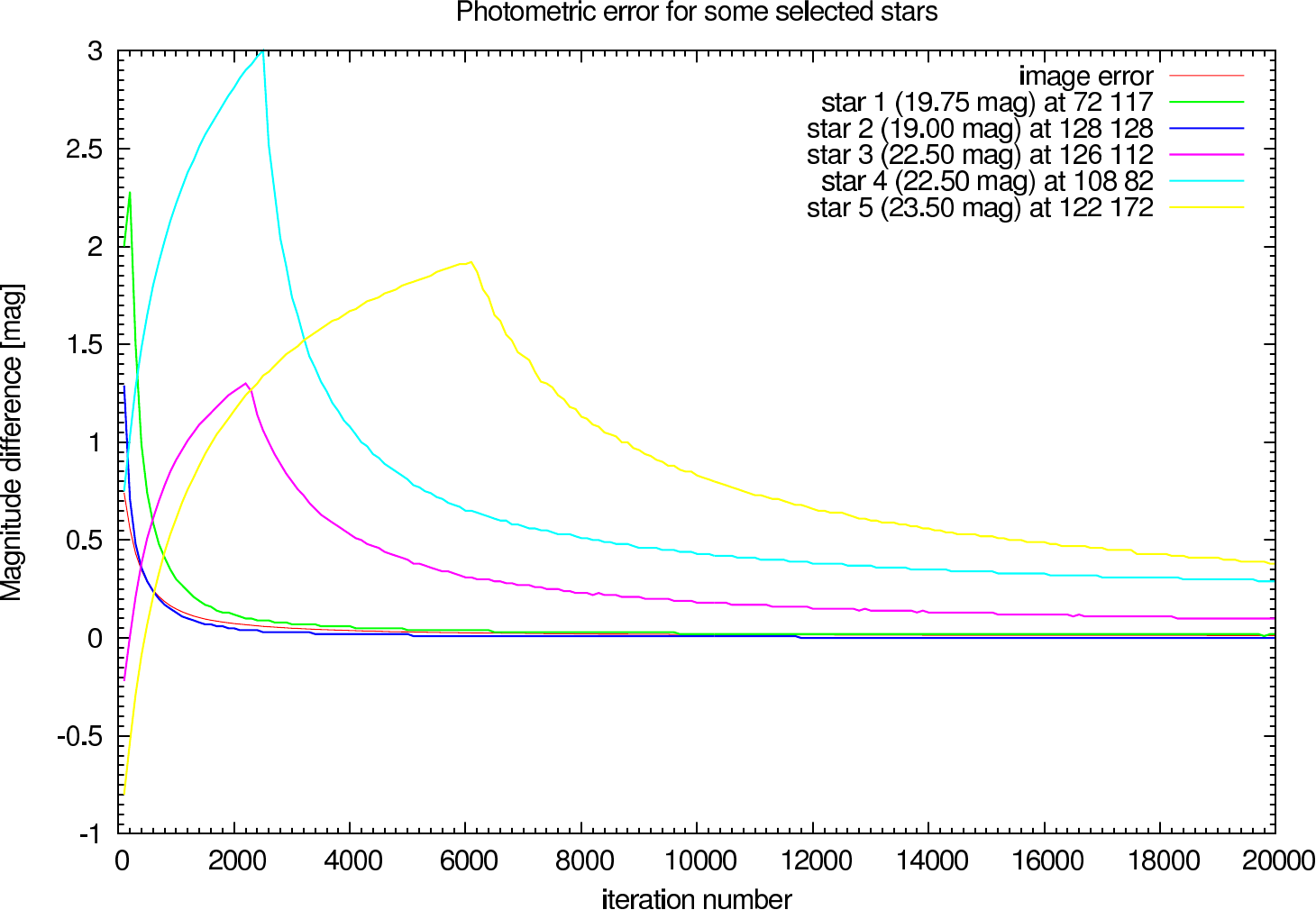
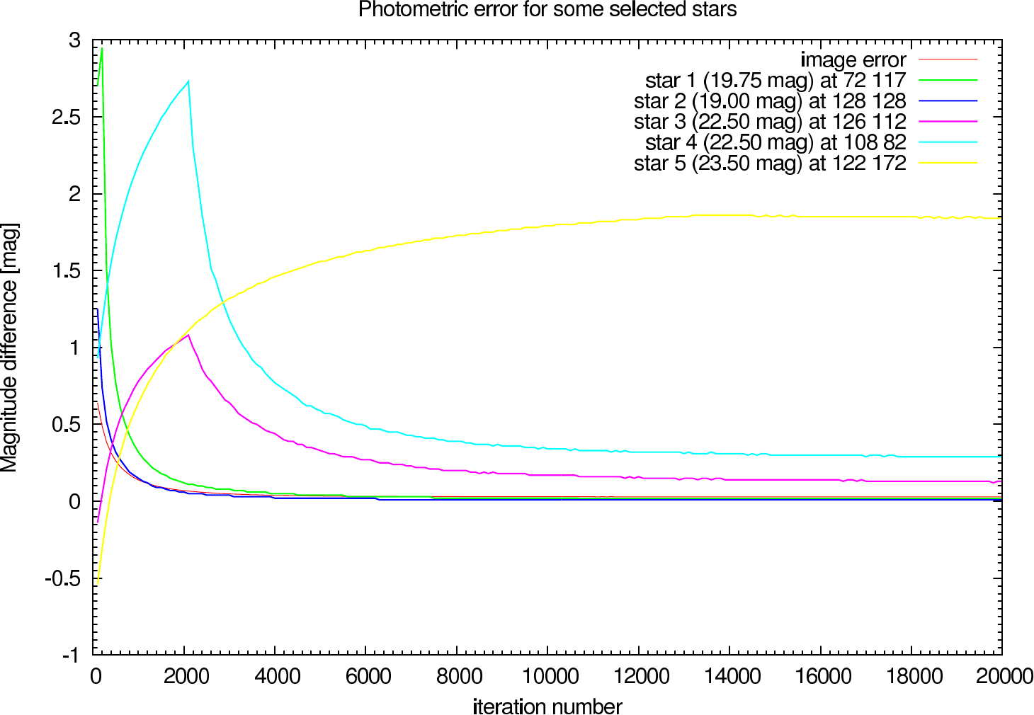
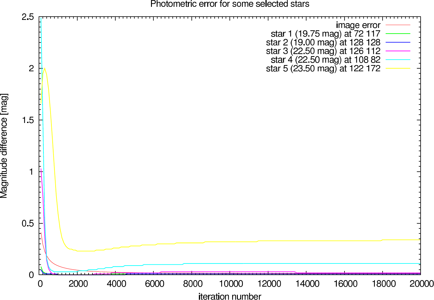
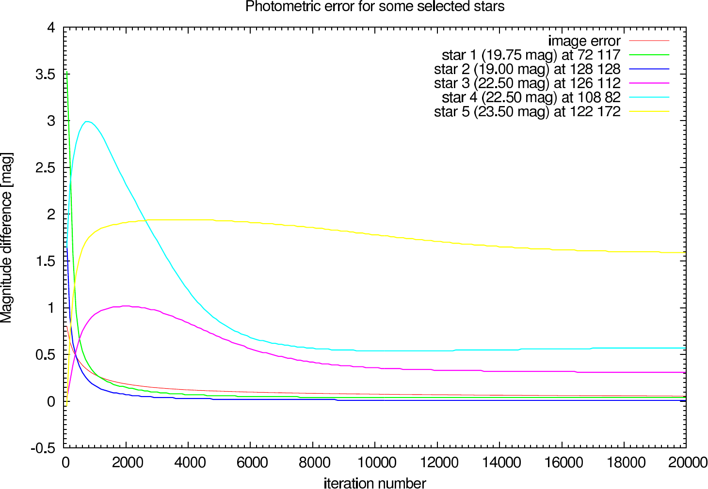
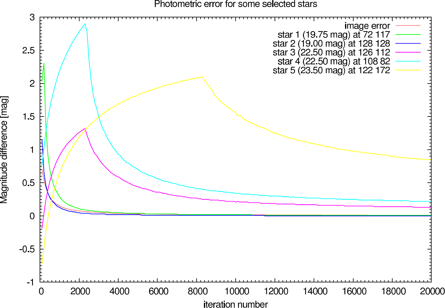
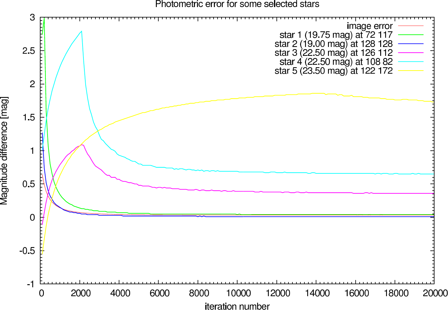
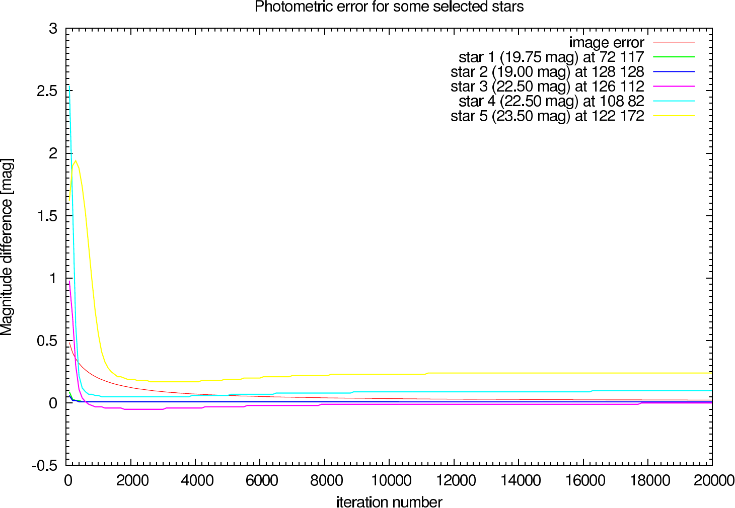
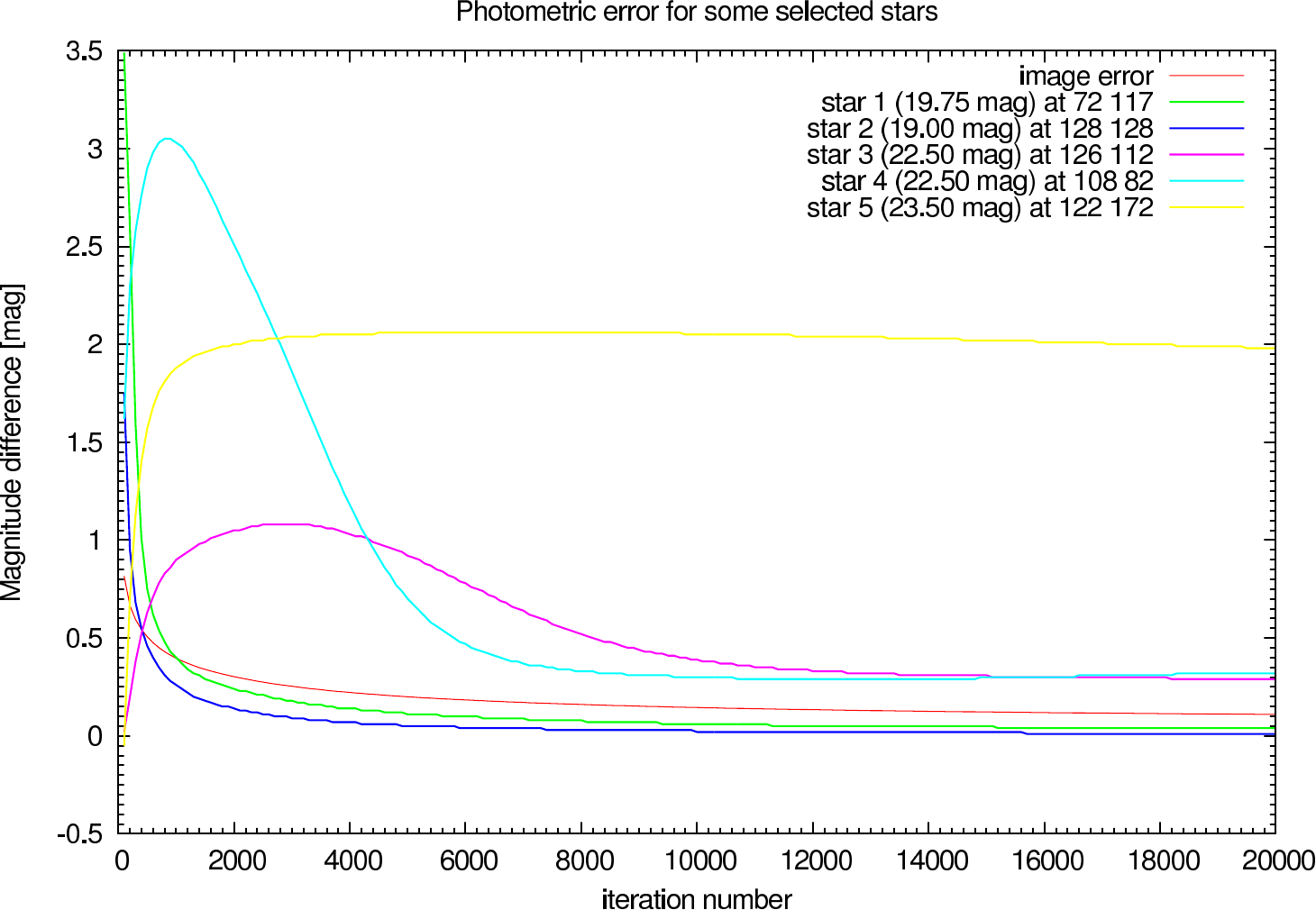
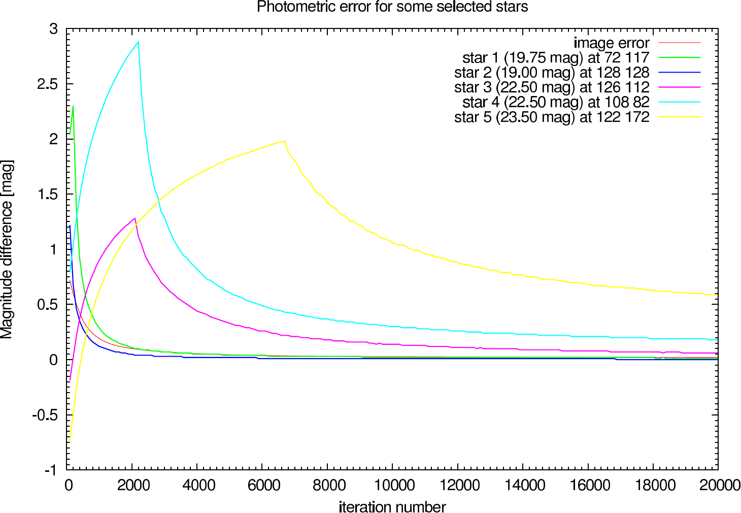
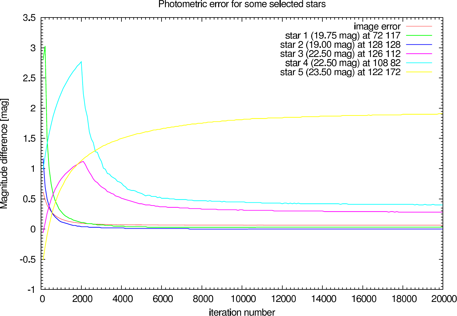
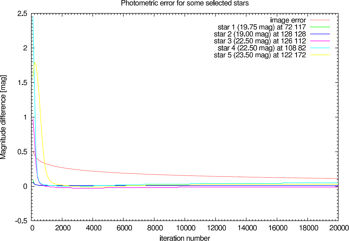
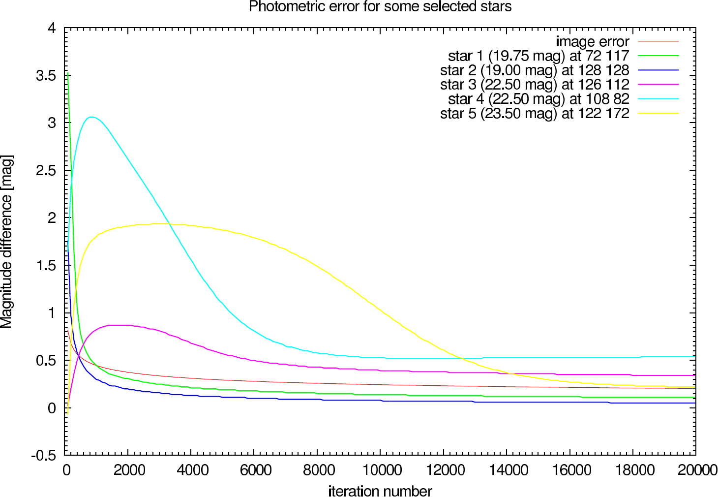
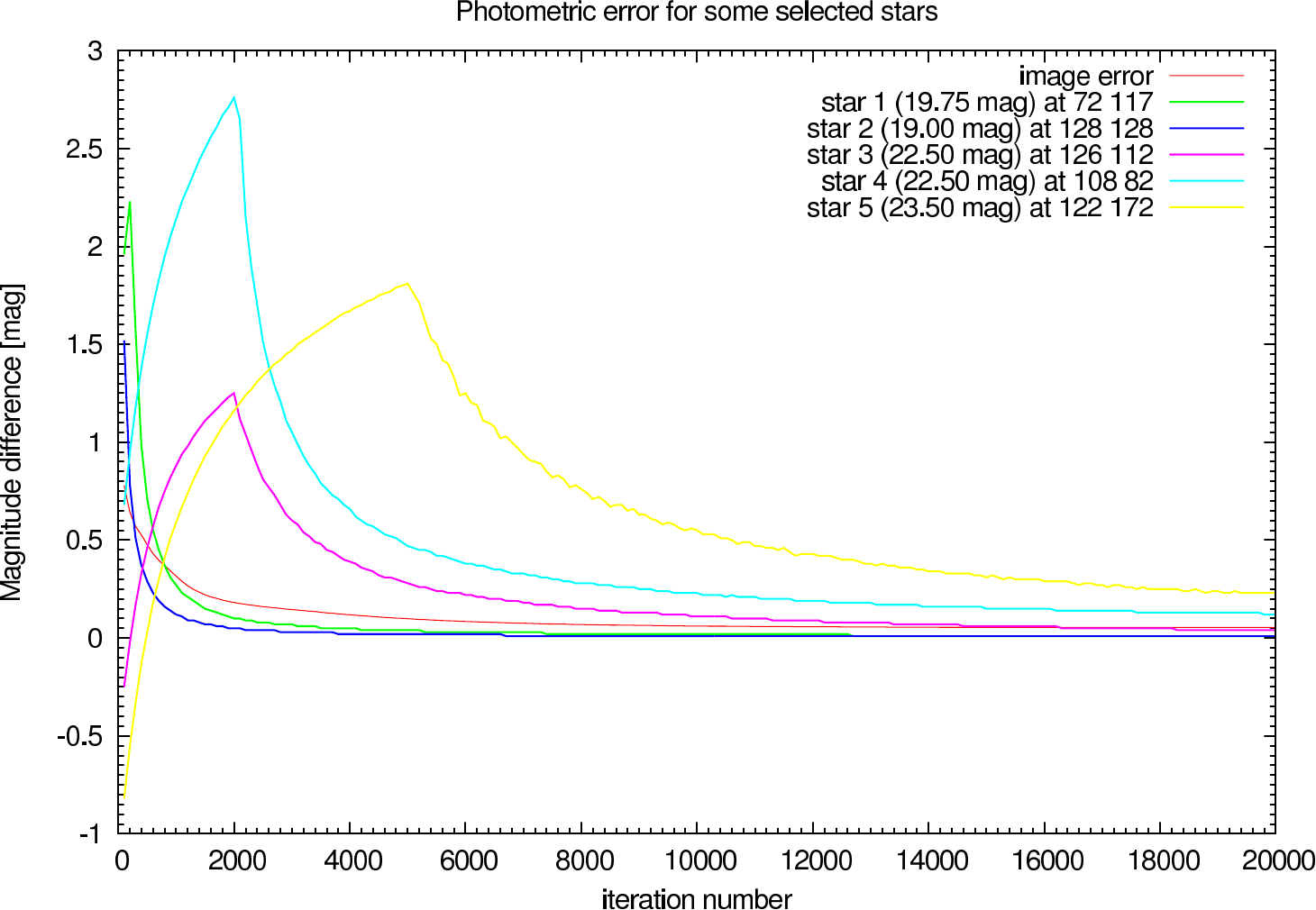
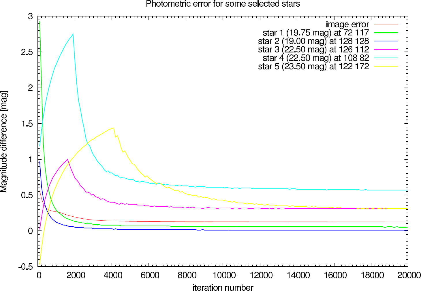
In the figures figure 15, figure 16, figure 17, and figure 18 the image and photometric errors depending on the calibrator strehl and the iteration number is shown. The overall shape is the same, but the optimum number of iterations is difficult to select, because not all photometric errors have their minimum at the same iteration number.

Figure 15: Image and photometric errors depending on the iteration number in the J-Band (left side) and K-Band (right side). The phase error is 0.0. For the reconstructions in the top row, Richardson-Lucy was used. In the second row, the Building-Block algorithm was used.

Figure 16: Image and photometric errors depending on the iteration number in the J-Band (left side) and K-Band (right side). The phase error is 0.1. For the reconstructions in the top row, Richardson-Lucy was used. In the second row, the Building-Block algorithm was used.

Figure 17: Image and photometric errors depending on the iteration number in the J-Band (left side) and K-Band (right side). The phase error is 0.2. For the reconstructions in the top row, Richardson-Lucy was used. In the second row, the Building-Block algorithm was used.

Figure 18: Image and photometric errors depending on the iteration number in the J-Band (left side) and K-Band (right side). The phase error is 0.5. For the reconstructions in the top row, Richardson-Lucy was used. In the second row, the Building-Block algorithm was used.