The Astronomical Image Processing System ( AIPS ) was developed by NRAO, originally to handle VLA data. It is now the most comprehensive radio image processing system available. You can not only use it for processing data optained by interferometers such as the VLA, WSRT, MERLIN, VLBA, EVN, VLBI you can also use it to work on single dish measurements and here the problem starts. Actually the variety of task (programs in AIPS) you can use to handle your radio data is sometimes confusing and on top of that you already need an idea what your radio measurements should look like.
This guide will help with your first steps in AIPS and hopefully will provide you with some confidence to calibrate your radio observations. More information and help can be found via the AIPS cookbook pages. However, once you have an idea of how AIPS works and what you should/can do with your radio data all other data processing packages use the same physical principles and are therefore easy to access even if the user interfaces appear different (e.g. Miriad ).
"The first steps" describes some basic features and useful tools in AIPS. "Get your hands dirty" will guide you through a complete calibration procedure. "AIPS advanced" will (still in development) provide some useful tips how to improve images, data massaging, combine UV-datasets, program run files.
Check if some AIPS ID numbers are reserved at your institute, if not just use a number of choice.
Figure out where your data files are, or just download a pre-preparted
UV-dataset or just have a look into the
VLA - archive and download some observations you are interested
in.
DOWNLOAD DAY1.CH0.UV.FITS (use right mouse bottom and save file)
A description how this file has been produced can be found here [ONLY for people which are familiar with AIPS].
If you would start AIPS from that directory where your data is stored,
the 'environment variable' which tell AIPS where to look for data is
set to PWD.
Tip: If you would like to load data or other files which are located in
a different directory than the one your have AIPS started in, you need
to set an environment variable before starting an AIPS session (e.g. setenv DATA /ftp/users/hrk/AIPS_MASTER_CLASS ).
Some other information will be shown which
can be ignored usually. However if AIPS fails to start
note any error messages, tape and disk numbers.
START_AIPS: Will start a new Unix Socket based TV

You have a choice of 10 printers.  These are:

    No. [ type  ] Description
-------------------------------------------------------------
     1. [     PS] Postscript printer, Tower L7, duplex
     2. [     PS] Postscript printer, Tower L8, duplex
     3. [     PS] Postscript printer, room 603, duplex
     4. [     PS] Postscript printer, room 614, duplex
     5. [     PS] Postscript printer, corridor near 614, duplex
     6. [     PS] Postscript printer, Tower L7, duplex
     7. [PS-CMYK] Tektronix colour printer, Tower L7
     8. [PS-CMYK] KMB only: HP deskjet colour printer
     9. [PS-CMYK] Postscript printer, transparencies
    10. [PREVIEW] Ghostview previewer
-------------------------------------------------------------

START_AIPS: Enter your choice, or the word QUIT [default is 10]: 10
START_AIPS: Your initial AIPS printer is the Ghostview previewer
START_AIPS:  - system name ghostview, AIPS type PREVIEW

START_AIPS: User data area assignments:
  (Using private file /home/ianh/.dadevs for DADEVS.PL)
   Disk 1 (1) is /data/ceardach/AIPS/DATA/ORNISH_1

Tape assignments:
   Tape 1 is REMOTE
   Tape 2 is REMOTE

START_AIPS: Starting TV servers on ornish asynchronously
START_AIPS:  - WITH Unix Sockets (new instance) as requested...
START_AIPS: Starting TPMON daemons on ORNISH asynchronously...
Starting up 31DEC05 AIPS with normal priority
Begin the one true AIPS number 1 (release of 31DEC05) at priority =   0
AIPS 1: ZDCHIN: NO NETSP ENTRY FOR DA02
AIPS 1: THIS MEANS THE TIMDEST LIMIT IS SET TO VALUE IN SP FILE OR 14.0
AIPS 1: You are not on a local TV device, welcome stranger
AIPS 1: You are assigned TV device/server  18
AIPS 1: You are assigned graphics device/server  18
AIPS 1: Enter user ID number
?UNIXSERVERS: Start TV LOCK daemon TVSRV3 on ornish
TVSERVER: Starting AIPS TV locking, Unix (local) domain
UNIXSERVERS: Start XAS3 on ornish, DISPLAY localhost:10.0
UNIXSERVERS: Start graphics server TKSRV3 on ornish, display localhost:10.0
UNIXSERVERS: Start message server MSSRV3 on ornish, display localhost:10.0
XAS: ** TrueColor FOUND!!!
XAS: Cannot use shared memory on remote XAS link
XAS: !!! Shared memory not selected !!!
XAS: Using screen width height 1270 924, max grey level 255

AIPS 1: Enter user ID number ?
You should get 3 new windows:AIPS_MSGSRV
Message server. Display only, it tells you how TASKS are working.
TEKSRV(Tek)
Tekserver for displaying b/w graphs etc. TEKSRV(Tek) will not appear till you use it.
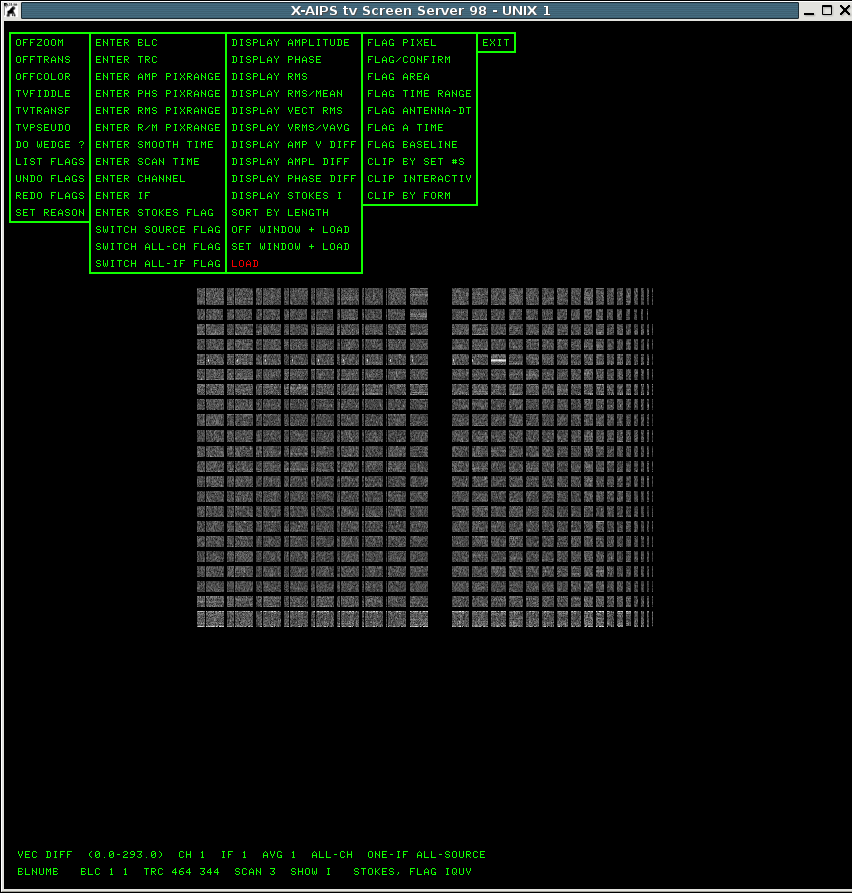
X-AIPS tv Screen Server 98
AIPS TV for coloured maps and interactive editing.
AIPS 1:                          31DEC05 AIPS:
AIPS 1:      Copyright (C) 1995-2005 Associated Universities, Inc.
AIPS 1:            AIPS comes with ABSOLUTELY NO WARRANTY;
AIPS 1:                 for details, type HELP GNUGPL
AIPS 1: This is free software, and you are welcome to redistribute it
AIPS 1: under certain conditions; type EXPLAIN GNUGPL for details.
AIPS 1: Previous session command-line history recovered.
AIPS 1: TAB-key completions enabled, type HELP READLINE for details.
AIPS 1: Recovered POPS environment from last exit
>
this command display all files in your (AIPS) disks (to specify the first diskindisk 1 , default is all [indisk 0])
AIPS 1: Catalog on disk  1
AIPS 1:  Cat Usid Mapname      Class   Seq  Pt     Last access      Stat
AIPS 1: Catalog on disk  2
AIPS 1:  Cat Usid Mapname      Class   Seq  Pt     Last access      Stat
Oxford specific: A machine that should run is hunda. In case you would
like to try it out
./MSSRV1: error while loading shared libraries: libsvml.so: cannot open shared object file: No such file or directory
./MSSRV1:: Too many arguments.
you need to edit some lines into you .cshrc or .alias files in your
home directories (look
here).
After the task has finished the message server will show the following output:
FITLD1: Task FITLD  (release of 31DEC05) begins
FITLD1: Found MULTI    observed on 11-MAY-1999
FITLD1: UV data will be written in compressed format
FITLD1: Create DAY1        .CH 0  .   3 (UV)  on disk  1  cno    1
FITLD1: Image=MULTI     (UV)         Filename=DAY1        .CH 0  .   3
FITLD1: Telescope=VLA                Receiver=VLA
FITLD1: Observer=AR405               User #=  333
FITLD1: Observ. date=11-MAY-1999     Map date=15-NOV-2005
FITLD1: # visibilities    976984     Sort order  TB
FITLD1: Rand axes: UU-L-SIN  VV-L-SIN  WW-L-SIN  BASELINE  TIME1
FITLD1:            SOURCE  FREQSEL  WEIGHT  SCALE
FITLD1: ----------------------------------------------------------------
FITLD1: Type    Pixels   Coord value     at Pixel     Coord incr   Rotat
FITLD1: COMPLEX      1   1.0000000E+00       1.00  1.0000000E+00    0.00
FITLD1: FREQ         1   8.1732000E+09       1.00  1.5625000E+07    0.00
FITLD1: STOKES       2  -1.0000000E+00       1.00 -1.0000000E+00    0.00
FITLD1: IF           2   1.0000000E+00       1.00  1.0000000E+00    0.00
FITLD1: RA           1    00 00 00.000       1.00       3600.000    0.00
FITLD1: DEC          1    00 00 00.000       1.00       3600.000    0.00
FITLD1: ----------------------------------------------------------------
FITLD1: Coordinate equinox 2000.00
FITLD1: Maximum version number of extension files of type HI is   1
FITLD1: Maximum version number of extension files of type FQ is   1
FITLD1: Maximum version number of extension files of type OF is   1
FITLD1: Maximum version number of extension files of type AN is   1
FITLD1: Maximum version number of extension files of type CL is   1
FITLD1: Maximum version number of extension files of type SU is   1
FITLD1: Maximum version number of extension files of type TY is   1
FITLD1: Maximum version number of extension files of type WX is   1
FITLD1: Appears to have ended successfully
check the disk and the files on it:
pca
AIPS 2: Catalog on disk  1
AIPS 2:  Cat Usid Mapname      Class   Seq  Pt     Last access      Stat
AIPS 2:    1  333 DAY1        .CH 0  .    3 UV 20-NOV-2005 12:29:06
Actually the header information provided via the fitld task can be obtained by typing
How AIPS stores the UV-datasets:
The file header AIPS files, like FITS files generally, have a header giving the important characteristics of the data. We normally process AIPS UV data in multi-source format (even single sources can be stored in this way). The results of calibration and editing in AIPS are stored in extension tables, along with more details of the data. The data itself is not modified so you can undo mistakes by deleting tables (although the data can be copied to another file with permanent corrections written into the data itself).
AIPS 1: Maximum version number of extension files of type HI is 1History table; inspect by typing
AIPS 1: Maximum version number of extension files of type AN is 1Antenna table; inspect by typing
AIPS 1: Maximum version number of extension files of type FQ is 1Frequency table, like all other tables can be inspected with the task 'PRTAB' but not very useful here.
AIPS 1: Maximum version number of extension files of type SU is 1Source table, can be inspected with the task 'PRTAB' and inext 'SU'. How to run a task and how to get the source information out of the dataset is topic of the next section.
Easy accessible information of your dataset is in the header. This information has been shown when you loaded the file into your AIPS disk. In case you have lost
that information
When was the observing run ?
11-MAY-1999
What kind of instrument are you using ?
VLA (actually it is D array, but you do not get that information check the VLA archive )
How many bands are you observing [IF] ?
2
How many polarisation are you observing [STOKES] ?
2
At which frequency are you observing [FREQ] ?
8.1732000E+09 Hz (this is only correct for IF 1)
Are these line- or continuum-observations [FREQ] ?
continuum with a 1.5625000E+07 Hz broad bandwidth
Now to get further information you first need to run the
getn 1
infile ''
cparm(3) 1
to see LISTR output
Usually sources and calibrators are marked. In case you are not familiar with any of the source names you can check the name and get some information about their structure via the VLA-calibrator database & explanation to the database to figure out which source is which.
To look at the inputs to the task PRTAB type:
AIPS 1: PRTAB:  Task to print any table-format extension file
AIPS 1: Adverbs     Values                 Comments
AIPS 1: ----------------------------------------------------------------
AIPS 1: USERID        0                    Image owner ID number
AIPS 1: INNAME     'DAY1'                  Image name (name)
AIPS 1: INCLASS    'CH 0'                  Image name (class)
AIPS 1: INSEQ         3                    Image name (seq. #)
AIPS 1: INDISK        1                    Disk drive #
AIPS 1: INEXT      'SU'                    Extension type
AIPS 1: INVERS        0                    Extension file version #
AIPS 1: BPRINT        1                    First row number to print
AIPS 1: EPRINT        0                    Last row number to print
AIPS 1: XINC          1                    Increment between rows
AIPS 1: NDIG          0                    > 3 => extended precision
AIPS 1: DOCRT        -1                    If > 0, write to CRT
AIPS 1:                                    > 72 => CRT line width
AIPS 1: OUTPRINT   ' '
AIPS 1:                                    Printer disk file to save
AIPS 1: DOHMS         1                    If > 0 print times with
AIPS 1:                                    hh:mm:ss.s format
AIPS 1: NCOUNT        0                    Print the first NCOUNT values
AIPS 1:                                    in a cell plus
AIPS 1: BDROP         0                    values BDROP through
AIPS 1: EDROP         0                    EDROP (if appropriate)
AIPS 1: BOX        *all 0                  List of columns to be printed
AIPS 1:                                    0 -> all.
You can get more information by typing
In some cases
will give you more details.
If the task was running without any problems the message server should have the following output.
PRTAB1: Task PRTAB  (release of 31DEC05) begins
PRTAB1: Appears to have ended successfully
PRTAB1: soay         31DEC05 TST: Cpu=       0.0  Real=       2
HELP/EXPLAIN taskname   help or more detailed help

APROPOS keyword         find appearance of keyword in all help files

ABOUT topic             list verbs, adverbs & tasks in topic category
INDISK n                access 'disk' (actually a directory) n

TASK 'taskname'         call 'new' task
(TGET taskname)         call an already used task
DEFAULT taskname        set all parameters back of the current task

INP                     list input parameters of current task

GO                      run a task
ABORT                   kill the task
CLRSTA                  clear status of a file
                        (do this after 'aborting' a task)
PCAT                    'ls' files (on current 'disk')
UCAT                    list UV files
MCAT                    list image files

GETN  m                 access file numbered m (on current disk) as infile
CLRN  m                 clear infile
GET2N m                 access file numbered m (on current disk) as in2file (need in2disk to be set)
CLR2N m                 clear in2file
GETON m                 access file numbered m (on current disk) as outfile (need outdisk to be set)
CLRON m                 clear outfile

ZAP                     delete file

RECAT                   renumber files (useful after deleting a file)

CLRMSG                  clear message server

IMHEAD                  view header

DOCRT 1                 change the help outprint from printer to terminal
move                    (task) move data to another user ID or copy data set
indxr                   (task) index a uv data base creates a new table (NX)
uvcop                   (task) copy part of UV dataset into a new file,
                               this is the only task that has no flag restriction.

prtab                   (task) print table
tabed                   (task) edit table
tacop                   (task) copy table

extdes                  (verb) delete table
prthi                   (verb)print history table (essentially all what you have done to the data)
SAVE mytask             save setting of the current task into mytask

GET mytask              call saved settings of mytask

SGDESTR mytask          deletes saved mytask

SGI                     list all saved mytasks

DEFAULT                 reset all parameter to default values (ONE TASK)

RESTORE 0               set all parameter values to default (ALL TASKS)

waittask ''             wait until task stop (useful to combine with various tasks
                        e.g. waittask 'indxr'; task 'uvplt';go)

for i = 1 to 2; getn i;clrsta;zap;end
                        loop that deletes file 1 and 2 on your disk

restart                 change between different user ID's
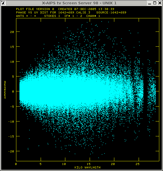
Emphasizing it, AGAIN the main body of a calibration effort is to identify bad data, edit the data by producing a FG table (flag table) and determine correction for the phase and the amplitude, which are stored in either an SN (solution table) or CL (calibration table) extension table.
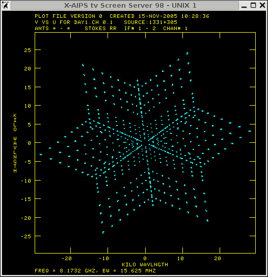
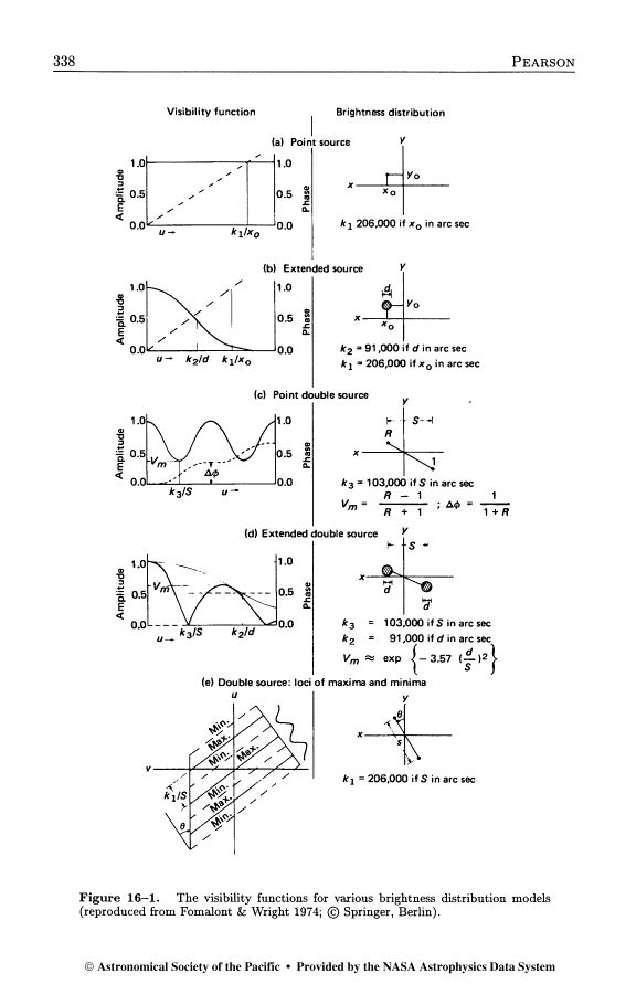
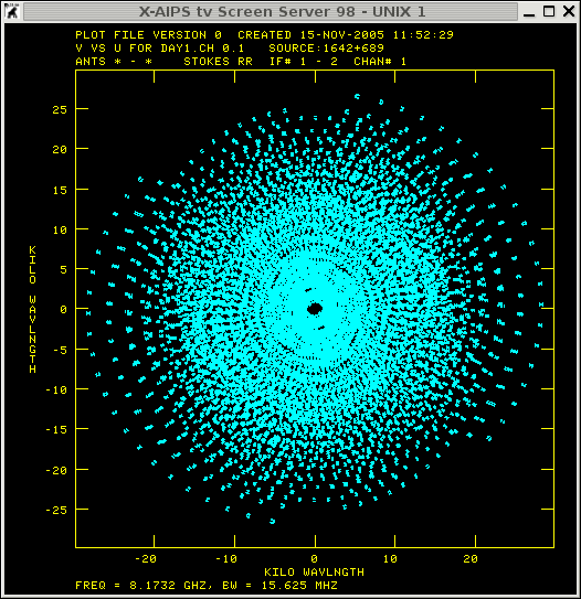
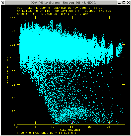
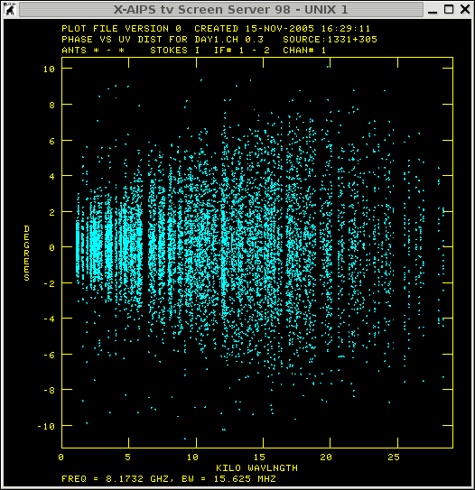
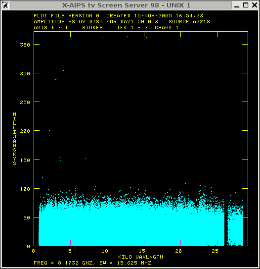
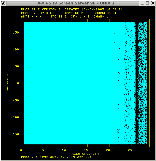
UV-coverage
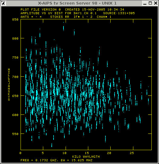
to get amplitude versus UV distance (this measurements should show a rather flat distribution).
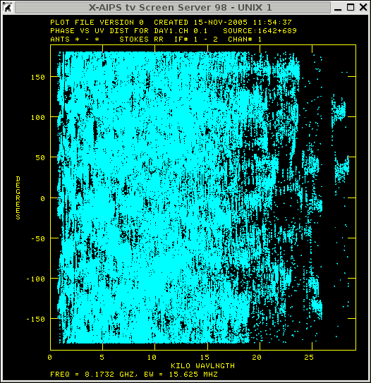
to get phase versus UV distance (for a calibrated point source it should be flat).
The next image provides you with a general idea of how the UV
distribution should look like for sources with different structures
[note that the sources are not in the phase centre, therefore you find
a changing phase with UV distance]
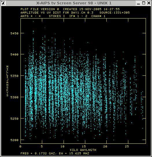
The UV data amplitude versus distance distribution does not reveal any strange amplitudes for this particular scan on 1331+305 (3C286), so finding systematic error on the basis of this source will not be successful.
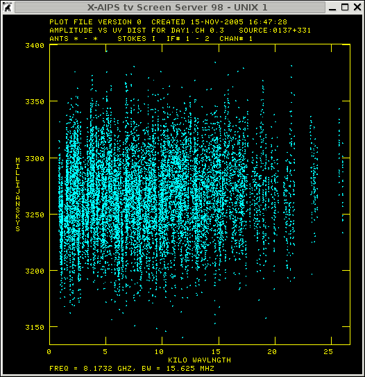
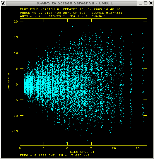
UV-plots for the 0137+331 (3C48)
Antenna based errors can be recognized by printing the system
temperature of each antenna versus time. In case there is no such
extension table the first CL table (I assume that the amplitude
calibration is included into this table) can be used.
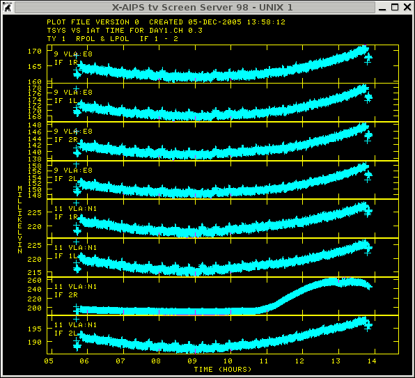
plot the Tsys measurements of the observation:
getn 1
inext 'ty'
timer 0 0 0 0 1 0
optype 'tsys'
source '''
nplots 8
Tsys (antenna 1 & 2, stokes R & L) versus time

|
Tsys (antenna 9 & 11, stokes R & L) versus time
|
The plots show the different system temperatures of the entire
observing run. The different temperatures at the begin and the end of
the observation is related to the amplitude calibrators, whereas the
small ripple during the run is the change of Tsys between
the target and the phase-reference source. The systematic errors we
are looking for are: the strange jump (antenna 1, IF 2, stokes R) at
around 13:00, the increase (antenna 11, IF 2, & stokes R) after
11:00. Actually there are some more recognizable errors which need to
be flagged (antenna 19, antenna 6 at around 6:15, antenna 28 around 13:10).
To produce a flag table one either can use uvflg or edita (this task
reads the Tsys measurements and will produce a flag table,
BUT it will not edit the ty table !).
the following commands will be used to produce a flag table:
getn 1
timer 0
antenna 19 0
stokes ''
flagv 1
timerang 0 6 10 0 0 6 20 0
timerang 0 12 58 0 0 13 41 0
timerang 0 10 20 20 0 14 0
stokes 'rr'
bif 2
eif 2
timerang 0 12 58 0 0 13 48 0
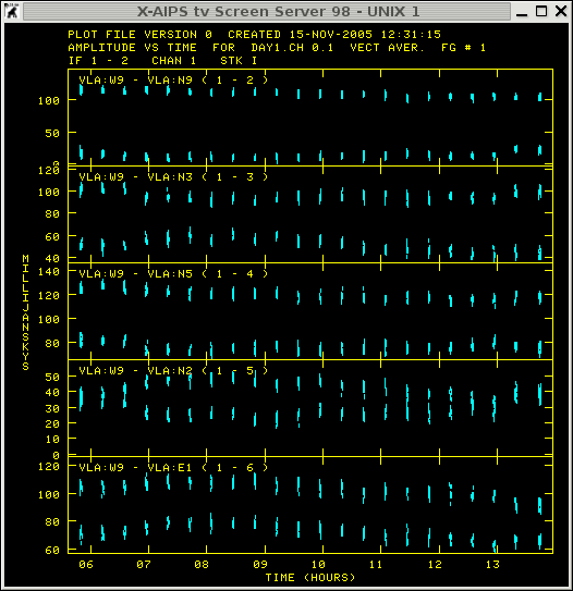
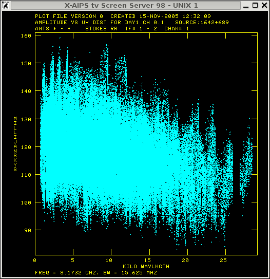
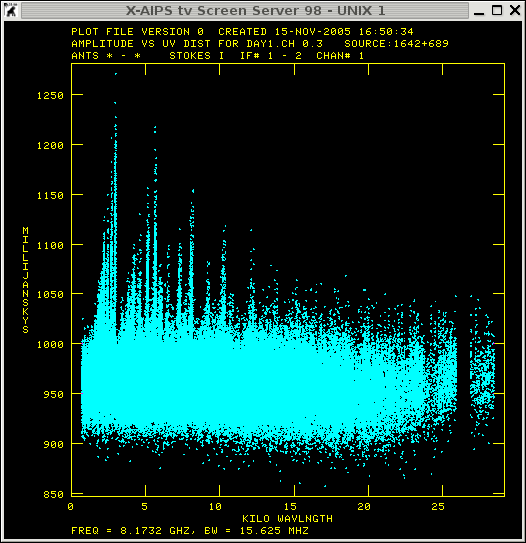
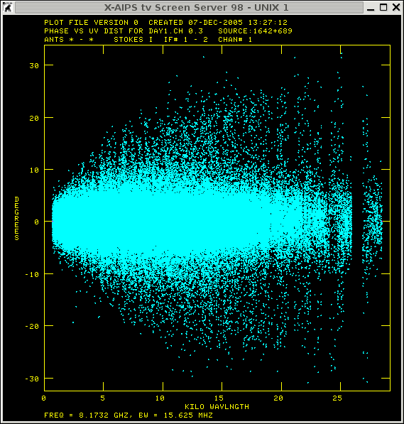
Baseline based errors can be spotted in investigating the measurements
of a calibrator source that has a simple structure and has been
observed frequently during the whole observing run (check LISTR output). For this purpose the source '1642+689' is ideal and will be
investigated.
plot the UV coverage of that source type:
getn 1
source '1642+689''
BPARM=6,7,2,0
UV-coverage
get amplitude versus UV distance (this measurements should show a rather flat distribution).
to get phase versus UV distance (for a calibrated point source it should be flat).
The amplitude versus UV-distance plot shows two distribution of points. In particular the points with decreasing amplitude versus UV-distance look suspicious and are worth for further investigation.
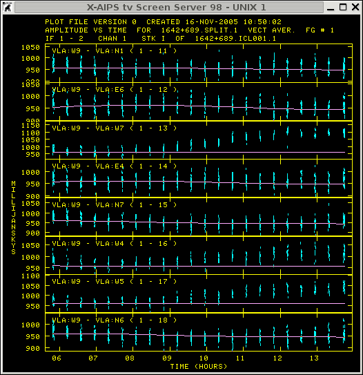
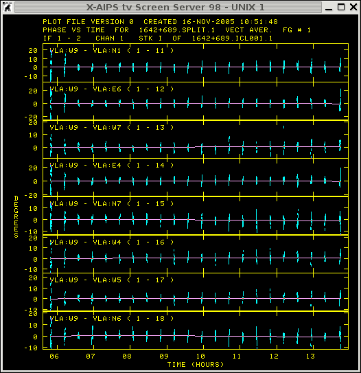
Another way to display the amplitude (or the phase) to reveal bad data is to plot these quantities versus time. This can be done for individual baselines with the task 'VPLOT'. For an interferometer with N Telescopes N(N-1)/2 baselines need to be inspected (VLA has 27 antennas so you need to check 351 baselines)! Note that you only look for systematics your are not flagging individual data points!
But before starting vplot it is important to know how the Telescopes are distributed to judge if some baseline show errors or just displaying the source sub-structures.
To check the telescope distribution use prtan for the VLA and for other observations visit the Observatory Homepages (EVN, VLBA, MERLIN, GMRT, WSRT, VLA, ATNF).
Now you are prepared to judge the following plots which display the amplitude versus time for both IF (that is the reason that for some baselines to 2 lines will appear).
getn 1
source '1642+689''
BPARM 0
nplots 5
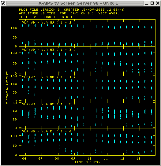
From the plot it seems that the data is strange for the first 10 seconds of each scan of that source. These are the systematic errors to look for! To flag this this kind of data one can use the task 'QUACK' to produce the first FG table. Note that no source will be specified, because we assume that this kind of error affects all the sources.
source ''
flagv 1
opcode 'beg'
aparm 0 10/60 0
In order to apply the FG table to the dataset the following input must be used in the future tasks:
Output task 'vplot' with FG table applied.
Output task 'uvpl' with FG table applied.
Further inspection of the data shows that antenna 28 behaves rather
strangely between 6:30 - 11:00 hours for the phase reference
calibrator and most likely for the target source. But this data should
NOT be flagged since the self-calibration procedure should be able to
correct for this kind of errors.
antenna.
Output task 'vplot' for some baselines of antenna 28.
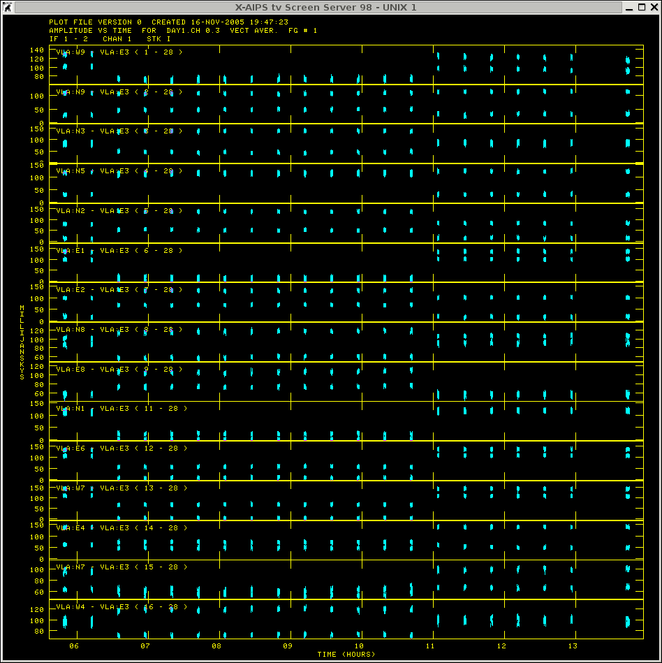
Apart from the strange amplitudes for antenna 28 the resulting UV distribution does not show any obvious systematic error anymore (Once again do NOT flag this data). After inspecting the other calibrators one can proceed to calibrate the observations.
1. Set the flux of the calibration source 1331+305 (3C286)
source '1331+305'
freq 1
bif 1
eif 2
aparm 0
optype 'calc'
SETJY1: Task SETJY  (release of 31DEC05) begins
SETJY1: A source model for this calibrator may be available
SETJY1: Use the verb CALDIR to see if there is one
SETJY1: A source model for this calibrator may be available
SETJY1: Use the verb CALDIR to see if there is one
SETJY1: / Flux calculated using known spectrum
SETJY1: BIF =  1 EIF =  2 /Range of IFs
SETJY1: '1331+305        ' IF =  1 FLUX = 5.3298 (Jy calcd)
SETJY1: '1331+305        ' IF =  2 FLUX = 5.2856 (Jy calcd)
SETJY1: / Using (1999.2) VLA or Reynolds (1934-638) coefficients
SETJY1: Appears to have ended successfully
SETJY1: soay         31DEC05 TST: Cpu=       0.0  Real=       0
The flux values of this source has been edit into the SU table.
2. Calibrate amplitudes and allow for minor phase correction. (note: The reference antenna should be one of the central antennas of the array.)
calsou '1331+305''
docalib 2
refant 6
aparm 4 0
doflag -1
soltyp 'L1R'
solmod 'A&P'
CALIB1: Task CALIB  (release of 31DEC05) begins
CALIB1: CALIB USING DAY1         . CH 0   .   3 DISK=  1 USID= 333
CALIB1: L1 Solution type
CALIB1: Selecting, editing and calibrating the data
CALIB1: Doing cal transfer mode with point model for each source
CALIB1: This is not self-calibration
CALIB1: Dividing data by source flux densities
CALIB1: Determining solutions
CALIB1: Writing SN table    1
CALIB1: RPOL, IF= 1 The average gain over these antennas is  2.793E+00
CALIB1: RPOL, IF= 2 The average gain over these antennas is  2.896E+00
CALIB1: LPOL, IF= 1 The average gain over these antennas is  2.785E+00
CALIB1: LPOL, IF= 2 The average gain over these antennas is  2.862E+00
CALIB1: Found          100 good solutions
CALIB1: Average closure rms =  0.0011 +-  0.0000
CALIB1: Fraction of times having data >  1.0 rms from solution
CALIB1: 0.50000 of the times had 26 - 28 percent outside  1.0 times rms
CALIB1: 0.25000 of the times had 28 - 30 percent outside  1.0 times rms
CALIB1: 0.25000 of the times had 30 - 32 percent outside  1.0 times rms
CALIB1: Appears to have ended successfully
→ SN 1 has been produced. Calib found 100 good solution indicating that there is not major problem with this dataset.
3. run calibrate on the other calibrator sources 1642+689 and 0137+331 (3C48).
calsou '1642+689''
CALIB1: Task CALIB  (release of 31DEC05) begins
CALIB1: CALIB USING DAY1         . CH 0   .   3 DISK=  1 USID= 333
CALIB1: L1 Solution type
CALIB1: Selecting, editing and calibrating the data
CALIB1: Doing cal transfer mode with point model for each source
CALIB1: This is not self-calibration
CALIB1: Dividing data by source flux densities
CALIB1: Determining solutions
CALIB1: Writing SN table    2
CALIB1: RPOL, IF= 1 The average gain over these antennas is  2.855E+00
CALIB1: RPOL, IF= 2 The average gain over these antennas is  2.964E+00
CALIB1: LPOL, IF= 1 The average gain over these antennas is  2.835E+00
CALIB1: LPOL, IF= 2 The average gain over these antennas is  2.917E+00
CALIB1: Found         2269 good solutions
CALIB1: Failed on       11 solutions
CALIB1: Average closure rms =  0.0020 +-  0.0001
CALIB1: Fraction of times having data >  1.0 rms from solution
CALIB1: 0.03409 of the times had 26 - 28 percent outside  1.0 times rms
CALIB1: 0.13636 of the times had 28 - 30 percent outside  1.0 times rms
CALIB1: 0.40909 of the times had 30 - 32 percent outside  1.0 times rms
CALIB1: 0.36364 of the times had 32 - 34 percent outside  1.0 times rms
CALIB1: 0.05682 of the times had 34 - 36 percent outside  1.0 times rms
CALIB1: Appears to have ended successfully
→ SN 2 has been produced.
calsou '0137+331''
CALIB1: Task CALIB  (release of 31DEC05) begins
CALIB1: CALIB USING DAY1         . CH 0   .   3 DISK=  1 USID= 333
CALIB1: L1 Solution type
CALIB1: Selecting, editing and calibrating the data
CALIB1: Doing cal transfer mode with point model for each source
CALIB1: This is not self-calibration
CALIB1: Dividing data by source flux densities
CALIB1: Determining solutions
CALIB1: Writing SN table    3
CALIB1: RPOL, IF= 1 The average gain over these antennas is  1.546E+00
CALIB1: RPOL, IF= 2 The average gain over these antennas is  1.613E+00
CALIB1: LPOL, IF= 1 The average gain over these antennas is  1.535E+00
CALIB1: LPOL, IF= 2 The average gain over these antennas is  1.587E+00
CALIB1: Found          103 good solutions
CALIB1: Failed on        1 solutions
CALIB1: Average closure rms =  0.0047 +-  0.0002
CALIB1: Fraction of times having data >  1.0 rms from solution
CALIB1: 0.25000 of the times had 28 - 30 percent outside  1.0 times rms
CALIB1: 0.25000 of the times had 30 - 32 percent outside  1.0 times rms
CALIB1: 0.25000 of the times had 32 - 34 percent outside  1.0 times rms
CALIB1: 0.25000 of the times had 34 - 36 percent outside  1.0 times rms
CALIB1: Appears to have ended successfully
→ SN 3 has been produced.
4. Set the flux of the phase calibrator sources in the SU table.
sour '1642+689''0137+331''
calsou '1331+305''
GETJY1: Task GETJY  (release of 31DEC05) begins
GETJY1:    Source:Qual      CALCODE IF  Flux (Jy)
GETJY1: 1642+689        :  0   A     1    0.95865 +/-   0.00425
GETJY1:                              2    0.95595 +/-   0.00414
GETJY1: 0137+331        :  0   A     1    3.26519 +/-   0.00696
GETJY1:                              2    3.22668 +/-   0.00624
GETJY1: Appears to have ended successfully
GETJY1: soay         31DEC05 TST: Cpu=       0.0  Real=       0
These flux measurements have been written into the SU table for the individual sources. However one should keep track of the estimated error of the amplitudes (save the output of the message server into a separate file). Since the source 0137+331 (3C48) is a well known flux calibrator source itself one could crosscheck the amplitude calibration.
5. Merge amplitude and phase solution from the individual SN tables into a CL table. For this step the task 'CLCAL' can be used.
This is a difficult 'and tricky' step since the absolute calibration has been done and the only source of interest is the calibrator that can be used to calibrate the target source, so in general one could skip calibrating the solutions of the other calibrator sources into a CL table. Tip: if there is no indication which source should be used for calibration compare the individual position of the sources with each other use the closest to calibrate the target source ( check LISTR output ).
However sometimes it is useful to have the calibration of the calibrator stored (e.g. if you are using the continuum data to calibrate the LINE dataset [to produce a bandpass, etc ...].) Therefore, the individual source positions have guide us to the following procedure to apply the calibration or better to produce the different CL tables:
produce CL table for 1331+305 only
sourc '1331+305''
calsou '1331+305''
opcode ''
refant 6
snver 1
inver 0
gainv 1
gainu 2
produce CL table for 0137+331 only
sourc '0137+331''
calsou '0137+331''
snver 3
gainv 1
gainu 3
produce CL table for 1642+689 and A2218
sourc '1642+689''A2218'
calsou '1642+689''
snver 2
gainv 1
gainu 4
Now check if the calibration improved the amplitudes and the phases of the individual calibrator sources.
|
getn 1 source '1331+305'' BPARM 0 docalib 2 gainu 2
|
amplitude
|
phase
|
|
getn 1 source '0137+331'' BPARM 0 docalib 2 gainu 3
|
amplitude
|
phase
|
|
getn 1 source '1642+689'' BPARM 0 docalib 2 gainu 4
|
amplitude
|
phase
|
|
getn 1 source 'A2218'' BPARM 0 docalib 2 gainu 4
|
amplitude
|
phase
|
The calibration of the short scan of the amplitude/phase calibrations are successful showing a rather linear relation between versus the UV distance. The UV distribution of the phase calibrator 1642+689 seem to show some strange spikes in amplitude at shorter baselines which can be corrected for in the self-calibration procedure.
After generating the different CL tables the UV dataset has been calibrated and one can write the individual source as single source file to disk. In case one find evidence for a large amount of data being bad, one would want to apply a better FG table to the phase calibrator and may perform the calibration steps again.
Example to write 1642+689 as a single UV-file:
source '1642+689''
stokes ''
docalib 2
gainu 4
aparm 0
Here we followed partially the Summary of AIPS Continuum UV-data Calibration from the AIPS cookbook.
The amplitude versus uv-distance plot of the source 1642+689 showed that there are some amplitude errors in the UV files. For the 351 baselines of these observations the task 'tvflg' can be used in order to visualize the calibrated UV dataset and to detect bad data.
getn 2
stokes 'i'
docalib -1
flagv 1
in the screen go to Display AMP V Diff, click left mouse button and if the colour is turning red type a
and then go to Load click on it and type a, then you should see.
The large amplitude variations are compensated by including the phase correction to the visibility. Apart from the few white point/horizontal lines indicating some bad times the data looks very good.
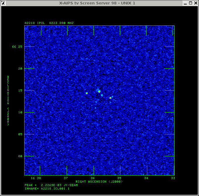
The final check of the data quality is to produce an images from the UV visibilities. The common task to do this is the task 'imagr'. This task is rather complicated and huge, therefore only a few step will be explained.
source ''
getn 2
imsize 256
go
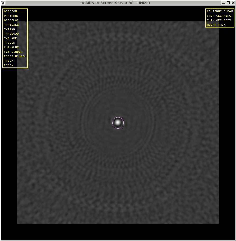
How to set a clean box.
| Click on TVBOX press a and then press c, then a, move mouse (with pressed left mouse button) to adjust for the radius of the clean box, press d. For rectangle clean boxes just skip pressing c. |
|
Within the cleaning process.
| This figure displays the clean process after subtraction (to get there type 3 times continue clean) 58 components (962.475 MilliJy). There is some residual component outside the clean box and one has to decide if these are real of caused by bad data. Note that this components are symmetric which could indicate some amplitude errors of a few baselines. |
|
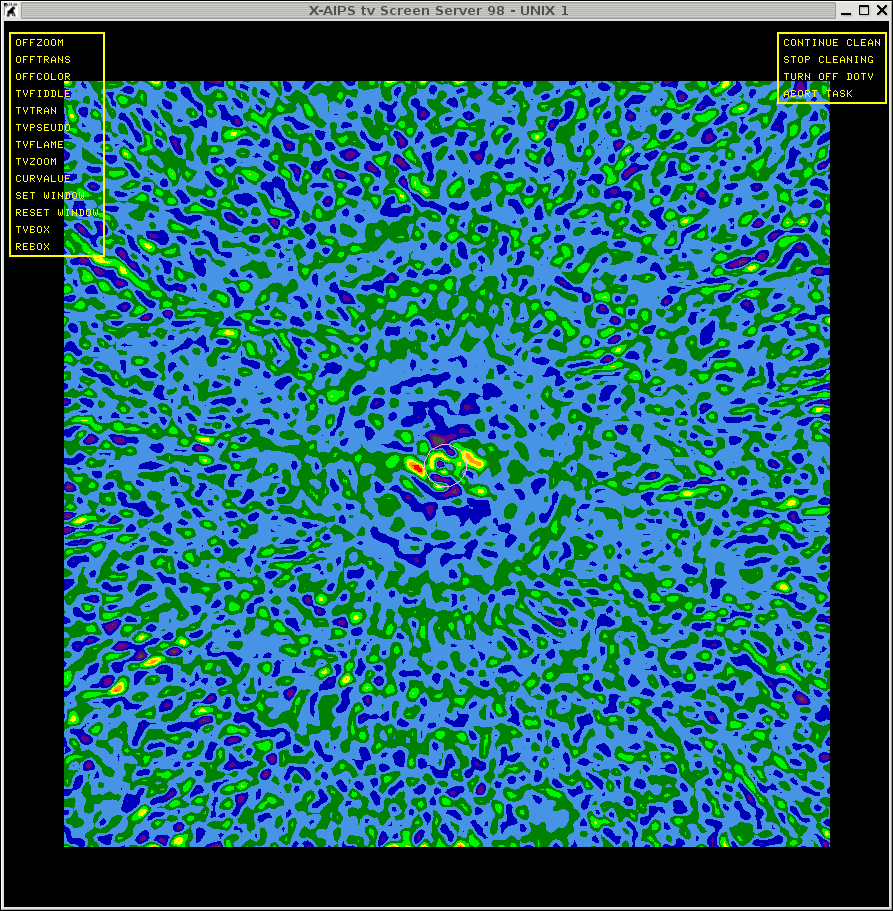
The task will stop after 500 iteration and will produce the final
image, which looks like the image below. It can be viewed by the following commands.
|
tvlo |
|
This image is far from being good and the radial pattern are residuals from the beam pattern which indicate some calibration errors.
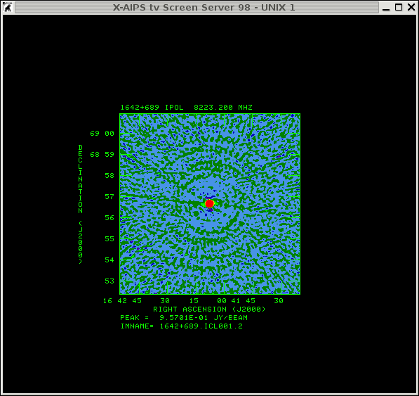
To get some statistical information on the image.
To determine the statistics choose a box excluding the source e.g. the lower part of the image.
AIPS 1: Set B.L.C. : button A, B, or C to change to T.R.C.
AIPS 1: Button D to kill and exit
AIPS 1: Set T.R.C. : button A or B to repeat B.L.C.
AIPS 1: Button C or D to exit
AIPS 1: BLC =    17.00   24.00    1.00    1.00    1.00    1.00    1.00
AIPS 1: TRC =   501.00  222.00    1.00    1.00    1.00    1.00    1.00
AIPS 1: Mean= 1.6832E-06 rms= 1.5717E-04 JY/BEAM   over   96515. pixels
AIPS 1: Maximum= 8.1135E-04 at   146   181    1    1    1    1    1
AIPS 1: Skypos: RA 16 42 48.594  DEC 68 54 07.45
AIPS 1: Skypos: IPOL  8223.200 MHZ
AIPS 1: Minimum=-7.9204E-04 at   30  101    1    1    1    1    1
AIPS 1: Skypos: RA 16 43 31.392  DEC 68 51 26.48
AIPS 1: Skypos: IPOL  8223.200 MHZ
AIPS 1: Flux density =  8.2158E-03 Jy.   Beam area =  19.77 pixels
A description of how to calculate the noise in an image is given in the VLA status summary .
Using the formulae (1) with K = 6.6 (for X-Band), N = 27 antennas (actually 26 antennas should be used); NIF = 2, the total time on source of around 22 x 3 minutes Tint= 1.1 hour, and Δνm = 2 x 15.625. Therefore, the expected noise in an naturally weighted image (so far we only produced uniform weight images but for the keen ones the image noise is 1.3252E-04 JY/BEAM; anyway it will provide an estimate if we have to do more) is 3.599E-05 JY. Comparing the theoretical estimate with the measured one of 1.5817E-4 JY/Beam means we are a factor of 4.4 off (that's not bad).
To find out what kind of problem could produce the higher noise in the image than theoretically expected, it is good to check the calibrated amplitudes and phases with the clean components of an image. This can be done with the task 'VPLOT'.
| These figures shows the measurements and the model (pink line, constructed from the clean components) versus time. As suspected from the image plane the amplitude of the data and the model does not agree on the baseline 1-13, 1-6, and 1-17 after 09:00 Hours and some more baselines. Note the data is more noisy (spread of points) in the first two scans. |
amplitude
|
phase
|
Despite the fact that more data massaging might have to be done for the phase reference source (essentially this should be done to understand the measurements in order to finally get your hands dirty on the target source) we can have a first look onto the target source A2218.
To split the UV-dataset and apply the calibration
source 'A2218''
stokes ''
docalib 2
gainu 4
aparm 0
source ''
getn catalogue number
cellsize 2
imsize 1024
niter 5000
dotv -1
The result of imagr is a cleaned image with 5000 clean components.
|
txinc 2 tyinc 2 tvlo |
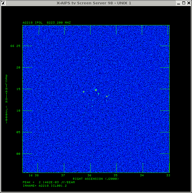
|
The noise estimates in the image is:
AIPS 1: BLC =    33.00   21.00    1.00    1.00    1.00    1.00    1.00
AIPS 1: TRC =   999.00  433.00    1.00    1.00    1.00    1.00    1.00
AIPS 1: Mean=-5.9647E-09 rms= 1.5627E-05 JY/BEAM   over  399371. pixels
AIPS 1: Maximum= 7.0729E-05 at   470   120    1    1    1    1    1
AIPS 1: Skypos: RA 16 36 00.786  DEC 65 59 43.67
AIPS 1: Skypos: IPOL  8223.200 MHZ
AIPS 1: Minimum=-7.1329E-05 at  704  416    1    1    1    1    1
AIPS 1: Skypos: RA 16 34 43.683  DEC 66 09 34.90
AIPS 1: Skypos: IPOL  8223.200 MHZ
AIPS 1: Flux density = -1.2840E-04 Jy.   Beam area =  18.55 pixels
The theoretical noise estimate is about 1.25342E-5 Jy, which is calculated with Tint= 6.825 hours. To get to the estimated noise one needs to do some self calibration (possibly first on the calibrator). Apply the new solutions to the target source and then do the same on the target source. How to do that will be covered in the AIPS advanced section.
Once one is satisfy with the data calibration here is the time to save
the file onto disk to have a backup (actually most of the data/calibration lost is due to either zapping the wrong file or deleting the wrong extension table).
getn 1
outfile 'PWD:DAY1.CH0.CALIB.UV.FITS'
This will produce a data file in the directory you have AIPS started from.
But before staring this chapter make sure that the previous steps of the
regular calibration has been done (amplitude calibration with an
external calibrator) and a first image has been produced of the
calibrator 1642+689.
|
amplitude versus UV-distance (1642+689)
|
cleaned image (1642+689)
|
From the previous sections it was already clear that the amplitude calibration step introduced some strange spikes at lower baselines and from the background pattern in the image showing symmetric errors (essentially the beam pattern) indicating these amplitude errors.
From now on the most important question is "What should be flagged ?" and the answer will be, almost nothing needs to be flagged!
Generally the first step in evaluating the image quality is to look
at the image background (cleaned) if there are some residual stripes
or symmetric pattern to see, which are present in this case. Depending
on the pattern and its symmetry one can judge the kind of error that
causes it. In general, the UV data or the visibility samples are
stored with amplitude and phase. Bad data is going to degrade the
image quality, so amplitude errors will produce a cosine error (even
or symmetric) and phase errors will produce a sinus error (odd or
unsymmetric) in the image plane (High Dynamic Range Imaging; Perley 1999, page 277
and Error Recognition; Ekers 1999).
One way of determine the image quality in a more qualitative way is
to use the dynamic range
(D=imagemax/rmsbackground). The catch is that it
is only possible to determine D if some prior knowledge of the UV
dataset is available. However generally for VLA observations the
following values provide an idea of the magnitude one would expect
(Perley 1999):
For the present observation of the calibrator source (1642+689)
the theoretical dynamic range can be estimated from the theoretical
rms 3.599E-05 JY and the flux estimates in the amplitude calibration
of 0.95865 JY (IF 1) to D = 26636. This dynamic range should be in
reach by using the self-calibration procedure only.
Another way in estimating the magnitude of the dynamic range (errors
confined to one baseline) is to use the simplistic formulae 13-9 in Perley 1999, page 279,
D=sqrt(M)sqrt(N(N-1))/phaseerror where N is the numbers of
antennas, M independent measurements (check with the task 'uvprt' for
the integration time which is 10 seconds). Phase errors are
commonplace from the atmospheric variation and are in the order of 10
degrees. Therefore the magnitude of the dynamic range will be of the
order of D=2522, 494, 95, for errors, effecting one baseline, one
antenna, all antennas respectively.
After amplitude calibration the dynamic range in the image of the
calibrator 1642+689 can be determine via the maximum flux in the image
(9.57E-01 Jy) and the estimated noise (1.4734E-04) leading to a
dynamic range of 6068. This already indicate that the measurement have
lower errors in phase.
The above formulae even they are simplistic are useful to estimate
how large have the phase and amplitude errors need to be to influence
the theoretical dynamic range.
To estimate the phases error the previous relation can be used the
other way around with D=26636. Therefore a phase error
phaseerror < 12.5 degrees [= 360/(2 •pi) •(351 •sqrt((2 •20+2 •3) •60/10.)/26636.)]
will not affect the dynamic range of the image.
To estimate the amplitudes errors a slightly different equation needs
to be used. In a naturally weighted image each sample has a weight of
1/Nsample. A single erroneous visibility with amplitude
amperror will cause an error sinusoid with a peak amplitude
of amperror/Nsample, which should be less than
the dynamic range.
amperror / Nsample < rmsbackground • imagemax
amperror < (N(N-1) •(2 •20+2 •3) •60/10.) • 3.599E-05 • imagemax
amperror < 6.9 imagemax
printing the amplitude, phase versus time 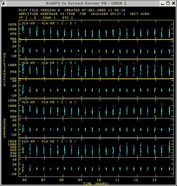 it seems that
the magnitude of the amplitudes and the phases are in the range of not affecting the
dynamic range in the image.
it seems that
the magnitude of the amplitudes and the phases are in the range of not affecting the
dynamic range in the image.
On be basis of the previous exercise no flagging should be done and one should proceed with the self calibration process.
In general, the self calibration process basically means focusing your image and the general procedure can be described like:
In case the dataset does not improve or the noise in the images does
not decrease one needs to investigate the data for bad baselines.
However in the case of the calibrator the general procedure did
not converge and the noise in the image essentially was in the order
of
In the following the first full step is described in the self-calibration process.
CALIB1: Task CALIB  (release of 31DEC05) begins
CALIB1: CALIB USING 1642+689     . SPLIT  .   1 DISK=  1 USID= 333
CALIB1: L1 Solution type
CALIB1: Create 1642+689    .CALIB .   1 (UV)  on disk  1  cno    5
CALIB1: Selecting the data
CALIB1: Doing self-cal mode with CC model
CALIB1: FACSET: 0.962445 Jy found from 81 components
CALIB1: Divide data by model - first compute model by summing
CALIB1: UVPREP: Maximum U Baseline is  2.806E+04 lambda.
CALIB1: ALGSTB: All   293 Rows In AP (Max    523)
CALIB1: ALGSTB: Ipol gridded model subtraction, chans    1 through    2
CALIB1: ALGSTB: Pass   1;  282-   0 Cells, with    82300 Pts
CALIB1: Field    1 used      81 CCs
CALIB1: Determining solutions
CALIB1: Writing SN table    1
CALIB1: Found         2269 good solutions
CALIB1: Failed on       11 solutions
CALIB1: Average closure rms =  0.0084 +-  0.0006
CALIB1: Fraction of times having data >  1.0 rms from solution
CALIB1: 0.05682 of the times had 34 - 36 percent outside  1.0 times rms
CALIB1: 0.22727 of the times had 36 - 38 percent outside  1.0 times rms
CALIB1: 0.50000 of the times had 38 - 40 percent outside  1.0 times rms
CALIB1: 0.21591 of the times had 40 - 42 percent outside  1.0 times rms
CALIB1: Applying solutions to data
CALIB1:            Previously flagged   Flagged by gain         Kept
CALIB1: Partially                 3350                3035      3350
CALIB1: Fully                        0                   0     78950
CALIB1: Copied OF file from vol/cno/vers  1    2   1 to  1    5   1
CALIB1: Copied AN file from vol/cno/vers  1    2   1 to  1    5   1
CALIB1: Copied WX file from vol/cno/vers  1    2   1 to  1    5   1
CALIB1: Appears to have ended successfully
CALIB1: soay         31DEC05 TST: Cpu=       1.9  Real=       2
|
phase versus UV-distance (1642+689)
|
after phase self-calibration
|
amplitude versus UV-distance (1642+689) 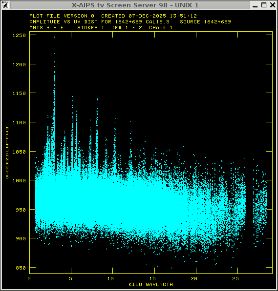 |
after amplitude self-calibration 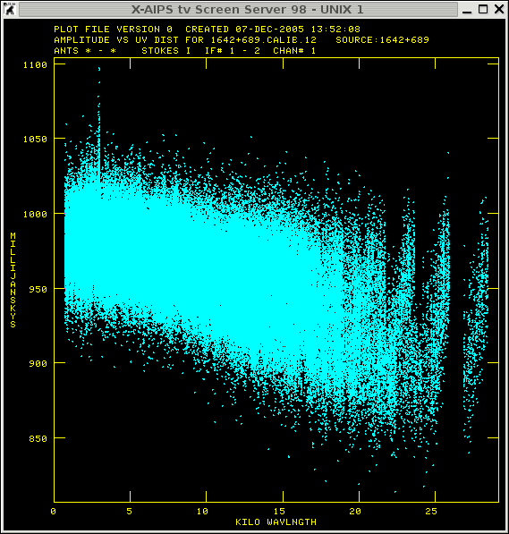 |
getn 2
and
sourc '1642+689''A2218'
calsou '1642+689''
opcode ''
refant 6
snver 4
gainv 4
gainu 5
Now apply the new calibration (CL 5) to the calibrator and produce a
new image. Sometime (also in this case) to your surprise the image
looks quite bad and the rms is high again
getn
Most of the differences between the two files appear in the first scan
and in the last so flagging these two scans for the calibrator do the
trick to get back to the lower noise levels.
Initially the purpose to calibrate the phase reference source was to
calibrate the target source with the improve amplitude and phase
corrections. To split the UV-dataset and apply the calibration
source 'A2218''
stokes ''
docalib 2
gainu 5
aparm 0
source ''
getn catalogue number
cellsize 2
imsize 1024
niter 5000
dotv -1
AIPS 1: Mean= 3.1487E-08 rms= 1.2851E-05 JY/BEAM   over  382389. pixels
AIPS 1: Maximum= 5.9809E-05 at   636   266    1    1    1    1    1
AIPS 1: Skypos: RA 16 35 06.249  DEC 66 04 35.37
AIPS 1: Skypos: IPOL  8223.200 MHZ
AIPS 1: Minimum=-6.3729E-05 at  666  353    1    1    1    1    1
AIPS 1: Skypos: RA 16 34 56.289  DEC 66 07 29.19
AIPS 1: Skypos: IPOL  8223.200 MHZ
AIPS 1: Flux density =  3.5744E-04 Jy.   Beam area =  33.68 pixels
The rms is very close to the theoretical estimates of 1.25342E-5 Jy and the target sources are to weak to self calibrate so we are done for the target source. However there is still some stuff one can do with the phase calibrator but I'm not going to do that at this stage.
For further reading Self-Calibration (Cornwell and Fomalot 1999). A good source on how to compute the theoretical noise can be found here (Wrobel and Walker 1999) and for any array specific values (e.g. system temperature) visit the homepage of the individual observatories.
To check whether the data of the observations are affected by that the AIPS task shado can be used. This task needs an antenna table as an input file which can be (downloaded here).
INFILE 'PWD:VLA-D.configuration
aparm 36 20 1 0
aparm(4)=-2
aparm(6)=1
go
Decl., deg  -2.   -1.    0.    1.    2.    3.    4.    5.    6.
    55.     1.00  1.00  1.00  1.00  1.00  1.00  1.00  1.00  1.00
    54.     1.00  1.00  1.00  1.00  1.00  1.00  1.00  1.00  1.00
    53.     1.00  1.00  1.00  1.00  1.00  1.00  1.00  1.00  1.00
    52.     1.00  1.00  1.00  1.00  1.00  1.00  1.00  1.00  0.93
    51.     1.00  1.00  1.00  1.00  1.00  1.00  1.00  1.00  0.93
    50.     1.00  1.00  1.00  1.00  1.00  1.00  1.00  1.00  0.89
    49.     1.00  1.00  1.00  1.00  1.00  1.00  1.00  1.00  0.89
    48.     1.00  1.00  1.00  1.00  1.00  1.00  1.00  1.00  0.89
    47.     1.00  1.00  1.00  1.00  1.00  1.00  1.00  1.00  0.89
    46.     1.00  1.00  1.00  1.00  1.00  1.00  1.00  1.00  0.89
    45.     1.00  1.00  1.00  1.00  1.00  1.00  1.00  1.00  0.89
    44.     1.00  1.00  1.00  1.00  1.00  1.00  1.00  1.00  0.89
    43.     1.00  1.00  1.00  1.00  1.00  1.00  1.00  0.89  0.85
    42.     1.00  1.00  1.00  1.00  1.00  1.00  1.00  0.89  0.85
    41.     1.00  1.00  1.00  1.00  1.00  1.00  1.00  0.89  0.85
    40.     1.00  1.00  1.00  1.00  1.00  1.00  1.00  0.89  0.85
    39.     1.00  1.00  1.00  1.00  1.00  1.00  1.00  0.89  0.85
    38.     1.00  1.00  1.00  1.00  1.00  1.00  1.00  0.89  0.85
    37.     1.00  1.00  1.00  1.00  1.00  1.00  1.00  0.89  0.81
    36.     1.00  1.00  1.00  1.00  1.00  1.00  1.00  0.89  0.81
This shows that the observations less than 43 degrees in elevation and an hour angle of 5 hrs will be affected by shadowing.
The elevation and the hour angle of the actual observation can be displayed via the task uvplt.
getn 1
stokes ''
freqid 1
source '1642+689''
bparm = 14 15 0
go
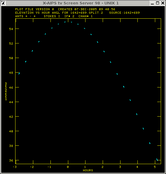 Indicating that the last scans of the phase
calibrator are affected by shadowing.
Indicating that the last scans of the phase
calibrator are affected by shadowing.
back to menu
However this section is ONLY for people who have experience in AIPS and know what kind of task can be used to facilitate in an automatic procedure.
The general structure is to have at least 2 procedures in a run
file. An example of a run file ( you
can download it here) is shown below. The first procedure in a RUN
file define the variables used in the following procedures. In this
particular case the AIPS tasks LISTR, PRTAN, and DTSUM will be started
after each other and the user can decide whether the output will be
printed on screen or on paper. Actually one can also choose to
get just the source info out of the dataset.
$ Comment:
$ This defines the variables for the procedure report

proc init_vars

SCALAR inputdisk, filenr, toscreen, dosource

finish
$
$ Comment:
$ This procedure will provide essential information of a multi source file
$
proc report(inputdisk, filenr)
$
toscreen=1;
dosource=1;
$
type 'Print on screen  ? [Yes 1 (default), No -1] --> 'read toscreen
type 'Only Source info ? [Yes 1 (default), No -1] --> 'read dosource
$
task 'listr'
indi inputdisk ; getn filenr ;
optype 'SCAN' ; inext ''; inver 0 ;
source '' ; calcode '' ; timer 0 ; stokes '' ;
selband -1 ; selfreq -1 ; freqid -1 ;
bif 0 ; eif 0 ; bchan 0 ; echan 0 ;
antenna 0 ; baseline 0 ;uvrange 0 ; subarray 0 ;
docalib 1; gainuse 0; dopol -1 ; blver -1 ;
flagv 0 ; doband 1 ; bpver 0 ;
smooth 0 ; dparm 0 ; factor 0 ; docrt toscreen ;
outprint '' ; baddisk 0 ;
go ; wait
if (dosource<0.0) then
$
task 'prtan'
indi inputdisk ; getn filenr ;
docrt toscreen ;
outprint '' ;
go ; wait
$
task 'dtsum'
indi inputdisk ; getn filenr ;
aparm 1 0 ;
docrt toscreen ;
outprint '' ; baddisk 0 ;
go ; wait
$
end
$
clrmsg
$
ret; finish
$
uvdata = AIPSUVData('MULTI', 'UVDATA', 1, 1)
- get some header informationuvdata.header.crtype[2]
uvdata.header.crval[2]- numbers of visibilities
len(uvdata)- address arrays
antennas[1:] = 2
ichansel[1][1] = 2
ichansel[1][1:] = [1, 2, 1, 0]
In addition the NEWS file from parseltongue-1.0.5 includes some useful tips how to do things.
Here is an example which does essentailly the same as the example above (download report.py).
#
# Get the PT anvironment
#
from AIPS import AIPS
from AIPSTask import AIPSTask, AIPSList
from AIPSData import AIPSUVData, AIPSImage
from Wizardry.AIPSData import AIPSUVData as WizAIPSUVData
#

# INITIALISE AIPS LOG FILE
AIPS.log    = open('./LOGFILE','a')
#
AIPS.userno =  5010
#

# This defines a function
def report(data,doprt='None'):
    """
    provide overview of the UVDATA file
    doprt expect STRING optional produce PS files.
    """
    noutput = -2
    # print scan list
    listr         = AIPSTask('listr')
    listr.indata  = data
    listr.optype  = 'SCAN'
    listr.docalib = 2
    listr.gainuse = 0
    if (doprt == 'None'):
        doprt = 'LISTROUTPUT'
    listr.outprint = 'PWD:'+str(doprt)
    listr.msgkill  = noutput
    listr.go()
    # print Antenna table
    prtan          = AIPSTask('prtan')
    prtan.indata   = data
    if (doprt == 'None'):
        doprt = 'PRTANOUTPUT'
    prtan.outprint = 'PWD:'+str(doprt)
    prtan.msgkill  = noutput
    prtan.go()
    # print dtsum for UV data file
    dtsum          = AIPSTask('dtsum')
    dtsum.indata   = data
    dtsum.aparm[1] = 1
    if (doprt == 'None'):
        doprt = 'DTSUMOUTPUT'
    dtsum.outprint = 'PWD:'+str(doprt)
    dtsum.msgkill  = noutput
    dtsum.go()

indata    = 1
inseq     = 1
uvdata    = AIPSUVData('G1','GMRTIN',indata,inseq)

printout  = 'PRINTOUT'

report(uvdata,printout)
Here you find a ParselTongue tutorial I gave at the ERIS in Oxford
2009 and all the examples are stored in a tar file HRK_PT_TUT.tgz.
|
|
if you have comments, suggestions or have spotted a dead link please let me know.
© H.-R. Klöckner 2005-2008