The Wythoff construction
Until now we have been concentrating more on the geometric properties of the regular
polyhedra and polychora and their regular compounds. However, as we will now see, a deeper
understanding of these objects can be gained by studying how they can be built from their
symmetries, in a process known as the Whythoff construction. This then makes it possible
to summarise all information on a polytope in an extremely compact and elegant way, its
Coxeter-Dynkin diagram. Apart from the improved understanding of polyhedra and polychora,
this will be important for understanding regular polytopes in higher dimensions, where the
geometric visualisation becomes difficult. This is meant only as a brief, non-technical
introduction, for a rigorous treatment see Coxeter (1973).
The Wythoff construction in 2D
The Wythoff construction is based on a very simple concept. In an object with, for
instance, bilateral symmetry, the left and right sides are identical, but appear as if
reflected in a flat mirror that goes through plane of symmetry of the object. Thus, in
this case, we could start with the right side of the object and obtain the left side by
reflecting it in that central mirror, generating the full symmetric object.
To a line associated with bilateral symmetry we add a second one perpendicular to it; in
the following Figures these are in light blue. These lines act as mirrors, which define a
specific kaleidoscope. These divide the plane
in four regions, which are the fundamental domains of this particular 2-fold dihedral symmetry,
which is a type of 2-D point symmetry
(i.e., a symmetry around a single central point).
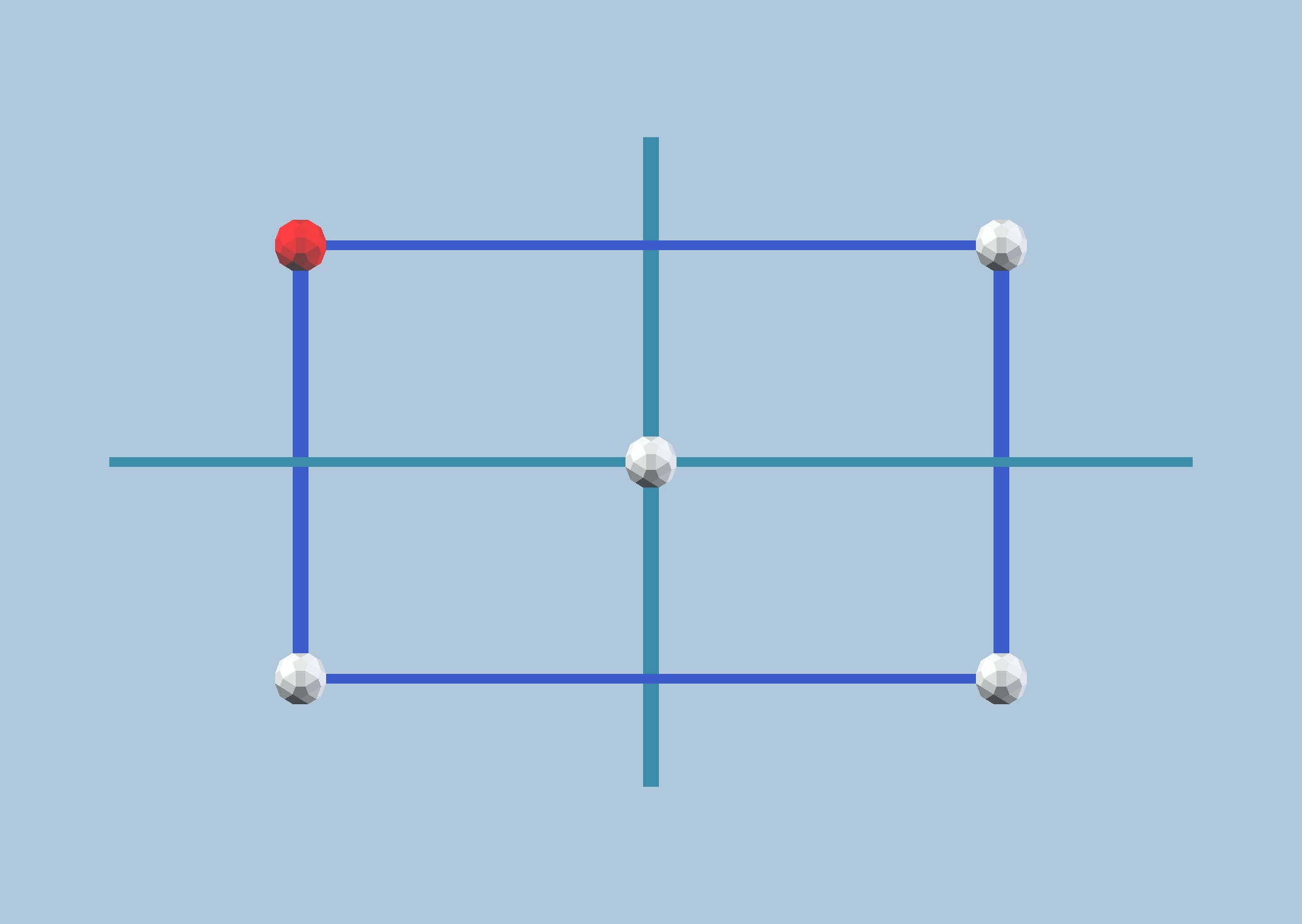
Fig. 9.1a: Two axes of bilateral symmetry define a 2-fold kaleidoscope. A point (in red)
has a total of three other reflections (in white), connecting them we obtain a rectangle.
Model made with vZome.
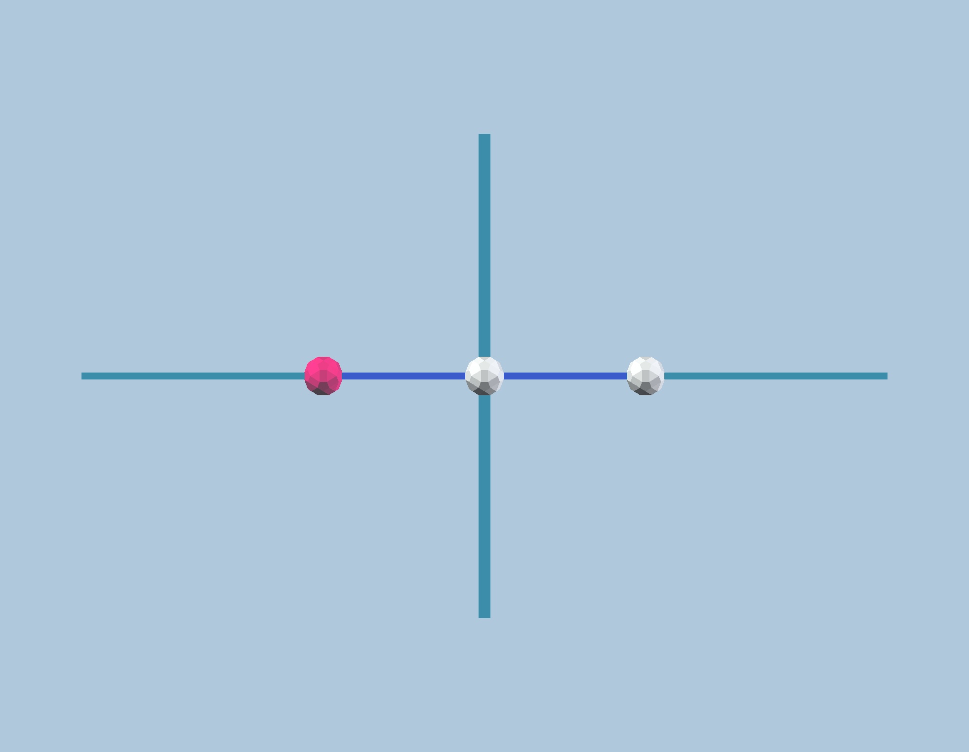
Fig. 9.1b: When a point is in one of the mirrors, it can only be reflected by the other
mirror. In this case, this lead to the formation of a digon. Model made with vZome.
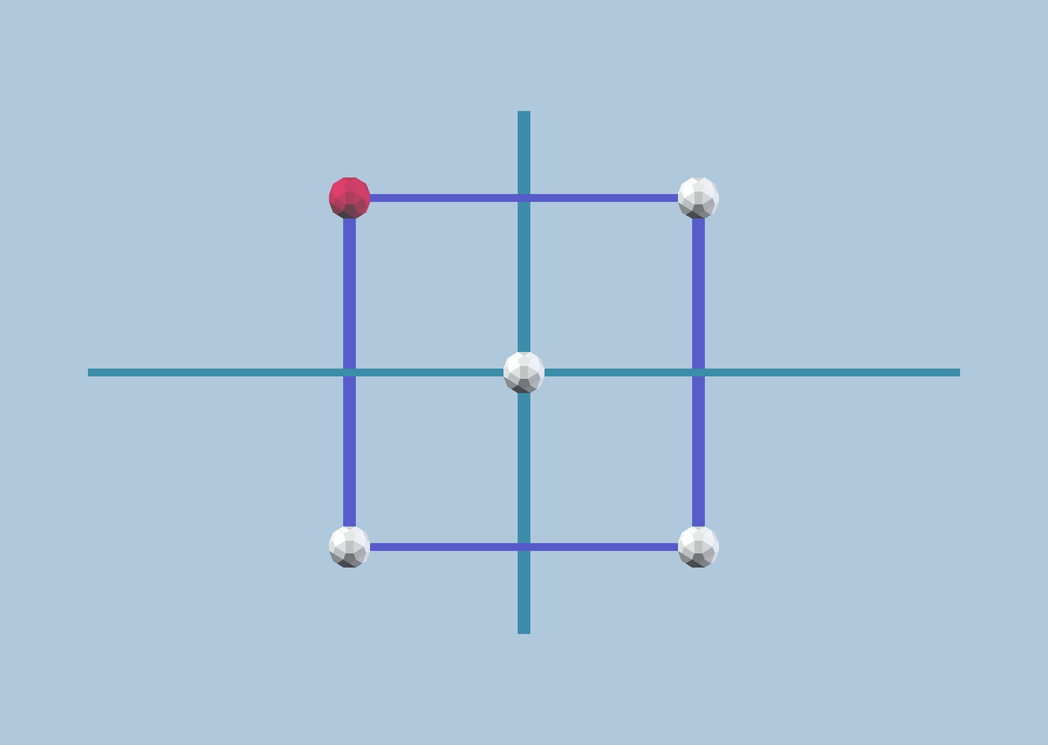
Fig. 9.1c: When a point is at the same distance from both mirrors, we obtain a Square.
Model made with vZome.
Now, here comes the important feature. Kaleidoscopes reflect a single object in the
fundamental domain into multiple copies. Our simple kaleidoscope in Fig. 9.1a does the
same: starting with one of the vertices (in red), we can use the two mirrors to create the
other three vertices. This is the basic idea of the Wythoff construction.
Connecting all vertices, we draw a rectangle. This figure has bilateral symmetry along two
different axes. This has an implication: we can rotate it by 360 / 2 = 180-degrees and the
figure will remain unchanged, something that does not necesarily happen for a figure with
bilateral symmetry only. This is an illustration of an extremely important feature of
these reflections, that they also define rotations
: an even number of reflections is equivalent to a rotation, and odd number of
reflections can always be expressed as a single reflection. This implies in general that
just by rotating a figure we cannot flip it!
In Fig. 9.1b, we highlight an important fact: when a point is in a mirror, it coincides
with its reflection by that mirror. The only noticeable reflection then is by a different
mirror, i.e., only one mirror (the one where the vertice isn't) is active. In this case,
the result is a 2-sided "polygon", a Digon.
In Fig. 9.1c, we reflect a point that is exactly in between the two mirrors. In this case,
both mirrors are active. This generates a Square, which has 4-fold symmetry.
All these figures have an important feature, central symmetry.
The same thing can be done to any regular Polygon: in the case of a Triangle, we can
choose a line going through its centre, one of its vertices and an opposing side that
divides it in two equal parts. Flipping the whole figure around this line leaves it
identical to itself (see Fig. 9.2a). This line is therefore an axis of bilateral symmetry.
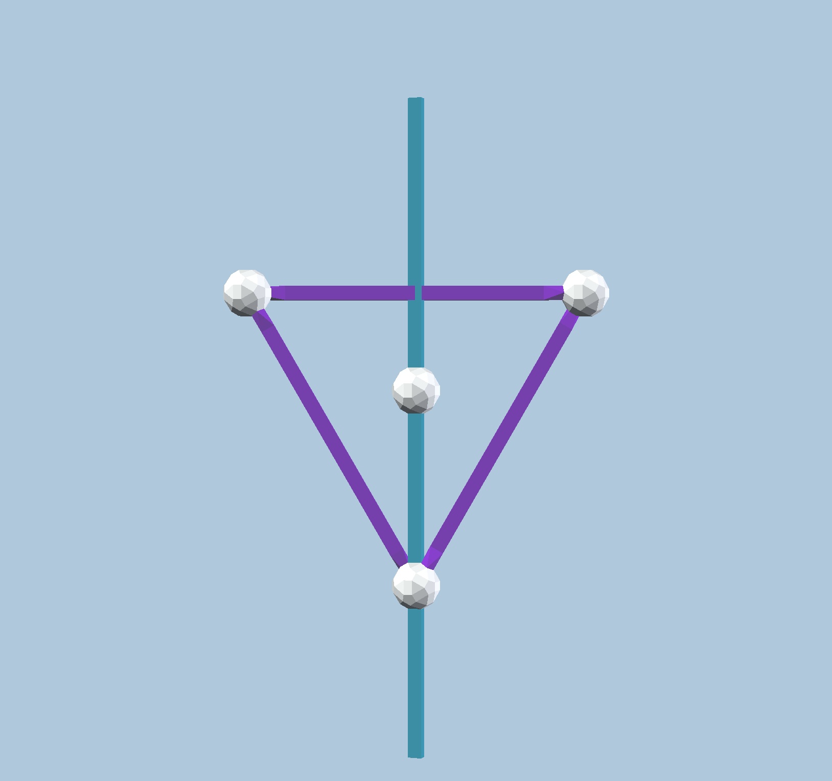
Fig. 9.2a: A regular triangle (in lavender color). The blue vertical axis defines one of
the lines of bilateral symmetry. Model made with vZome.
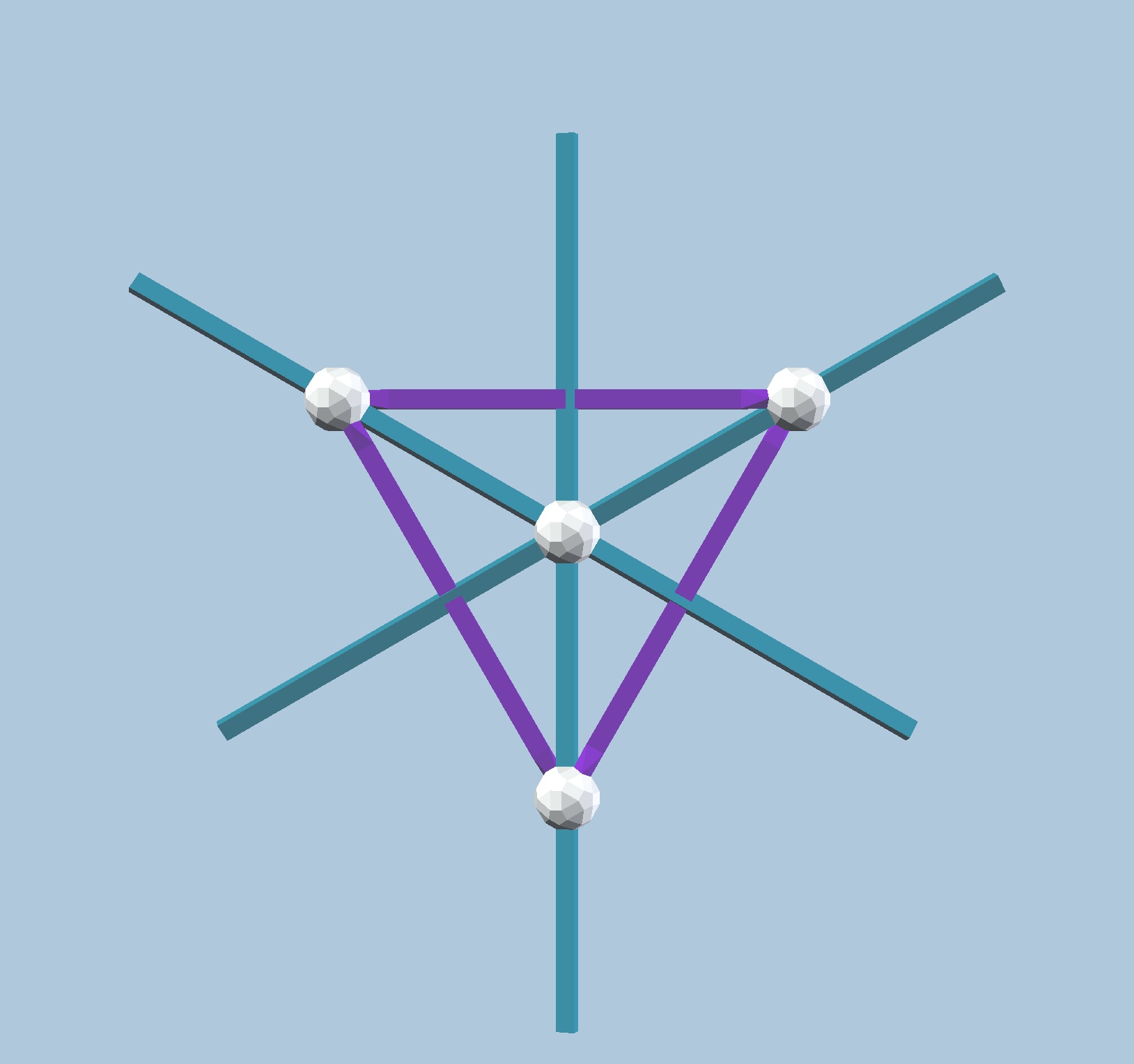
Fig. 9.2b: A Triangle has two more such axes of bilateral symmetry. These define the
kaleidoscope of the 3-fold dihedral symmetry, where the plane is divided in six regions.
Model made with vZome.
However, it should be clear that the Triangle has two other such lines, which cross at the
centre of the triangle (Fig. 9.2b) They create six separate regions in the plane, which
are defined by angles of 180 deg / 3 = 60 degrees, these are the fundamental regions of
the 3-fold dihedral symmetry. Note that this symmetry has no central symmetry!
As before, different positions of initial points result in different figures. In Fig.
9.3a, moving the initial vertex from a point in an axis of bilateral symmetry to its
neigbour, we create the dual Triangle, in red, i.e., we switched which mirror is active.
For a point in the middle of the fundamental region, both mirrors are active, createing a
regular polygon with 2n sides, in this case a Hexagon (Fig. 9.3b). If the initial point is
not exactly at the same distance from the two mirrors, we create an irregular Hexagon,
like the ditrigon in Fig. 2.3e. These represent different types of Wythoff construction
acting on the same kaleidoscope.
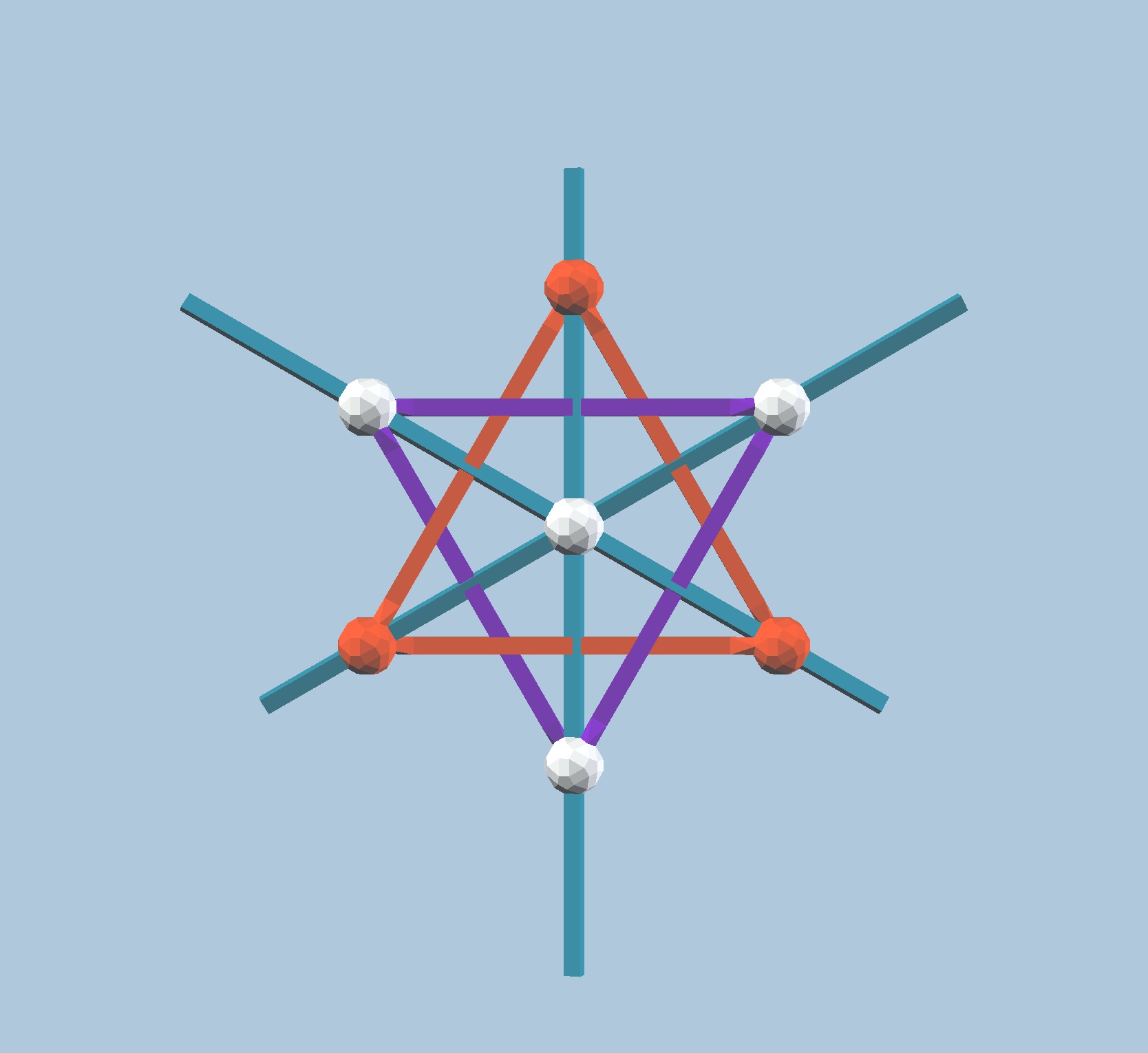
Fig. 9.3a: A point located in a neighbouring axis of bilateral symmetry creates a dual
polygon, in red. Model made with vZome.
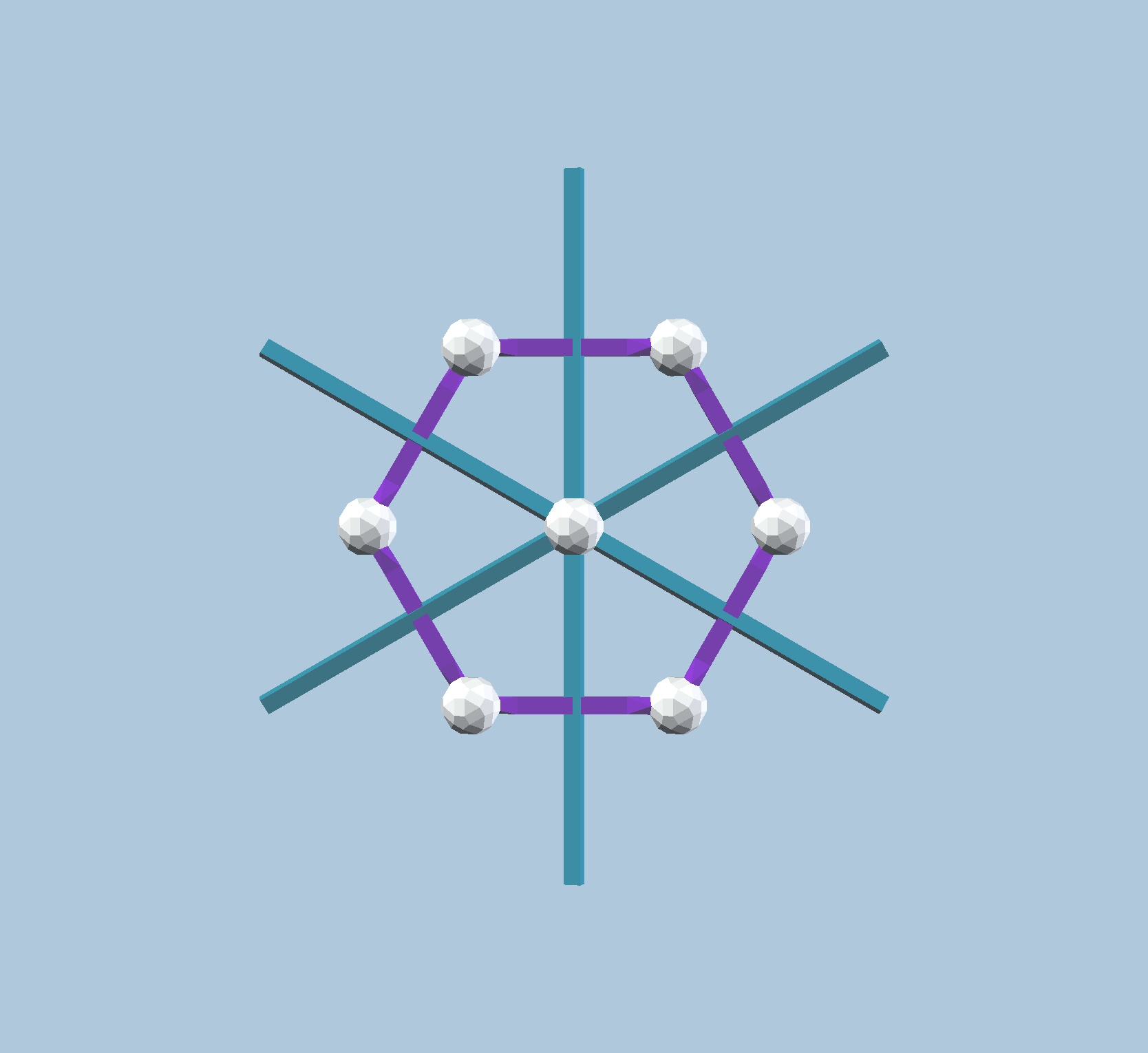
Fig. 9.3b: A point equidistant from the axes of bilateral symmetry produced a regular
polygon with 2n sides.
The Square and Hexagon can, of course, also be obtained from 4-fold and 6-fold dihedral
symmetry. The fact that they can also be derived from the 2-fold and 3-fold ditrigonal
symmetries is a general feature of the Wythoff construction: in many cases, the same
polytope can be obtained by different Wythoff constructions in different underlying
kaleidoscopes.
The Wythoff construction in 3D
We will now build the Kaleidoscopes associated with the regular polyhedra. The starting
idea is the same: we start by looking for the planes of bilateral symmetry for the whole
polyhedron, which go necessarily through the the centre of the whole figure. The full set
of such planes then defines the 3-D polyhedral kaleidoscope, where they act as mirrors.
For a particular regular polyhedron A, it is clear that its planes of bilateral symmetry
must go through its edges: each edge separates two identical faces, from each of these A
looks identical. However, it is also true that the edges connect two identical vertices,
from which A also looks identical. This implies that the lines perpendicular to the edges
- the edges of the dual of A, here designated B, must also be coincident with planes of
bilateral symmetry. Thus, all edges of the dual polytope compounds in Fig. 3.3a, b, and c
are in the planes of bilateral symmetry of the dual pairs A/B.
However, looking at those figures, it is clear that the planes of bilateral symmetry
define a further set of edges. To see them, we need to extend each edge "around" the
polyhedron, making it an equatorial polygon. To do this, we add to the edges in models in
Figs. 3.3a, b and c the edges used in making the Cube and other rhombic polyhedra. Doing
this, we achieve a representation of the kaleidoscopes of the regular polyhedra, these are
displayed in the next Figures.
Why specifically the rhombic polyhedra, and not the quasi-regular polyhedra, which are
also isotoxal? The reason is that the rhombic solids are isohedral, thus the edges between
faces must also be in the planes of bilateral symmetry.
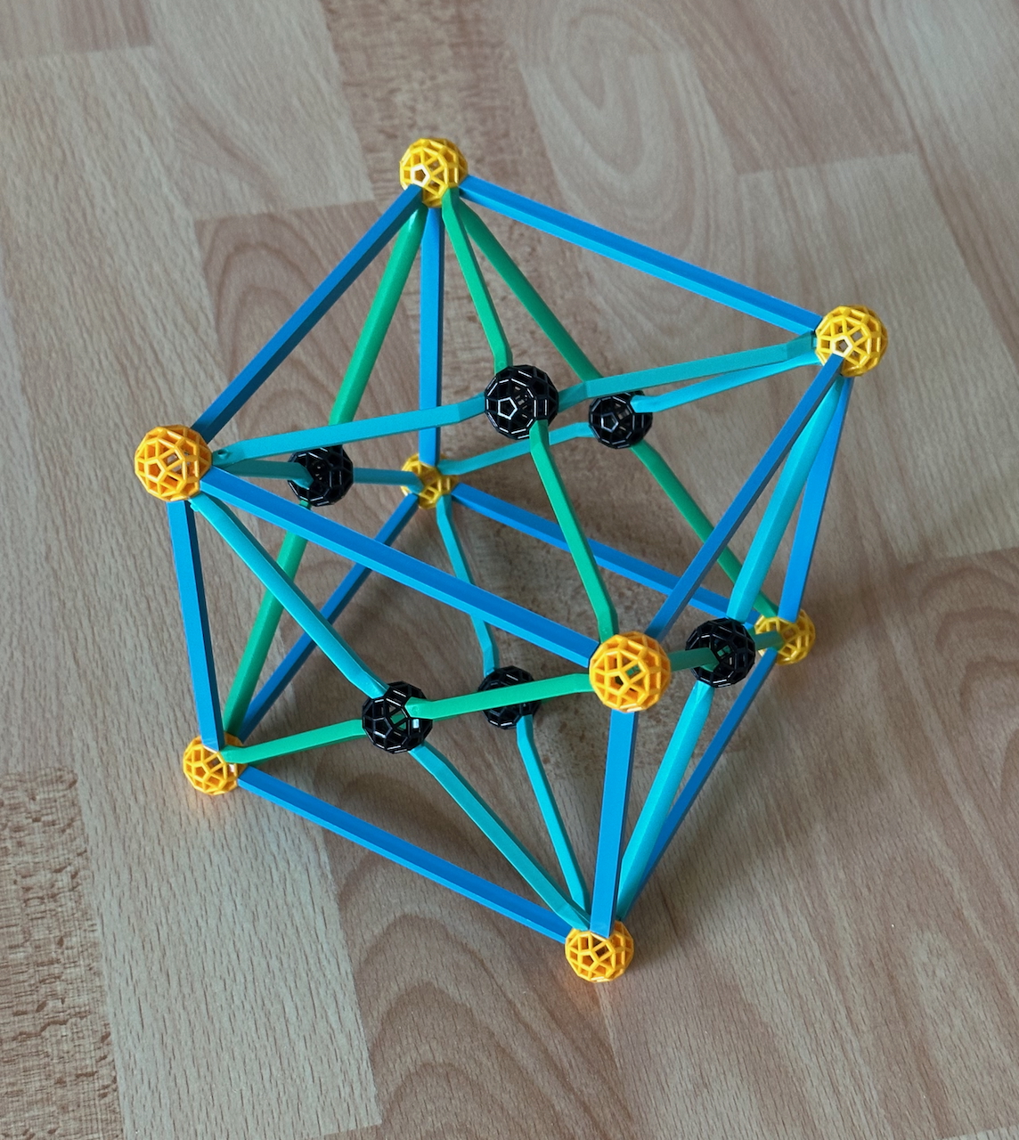
Fig. 9.4a: The Tetrahedral kaleidoscope. The Tetrahedron is represented by the green HG2
struts, the other struts are there only to represent planes of bilateral symmetry.
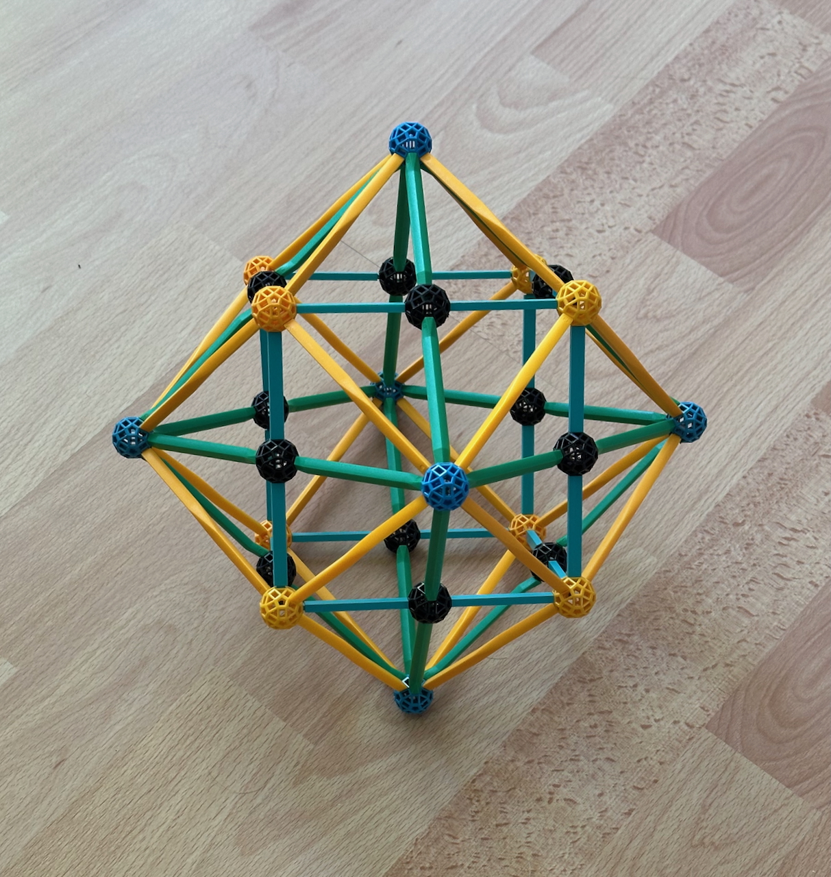
Fig. 9.4b: The Octahedral kaleidoscope. In this model, we used HG2 struts for the edges of
the Octahedron and half-blue 2 struts (in teal) for the edges of the Cube. The latter HB
struts are very rare and unfortunately no longer made by the Zometool company. Using HB
and HG struts allows the use of a single Y2 strut to represent the edges of the Rhombic
dodecahedron.
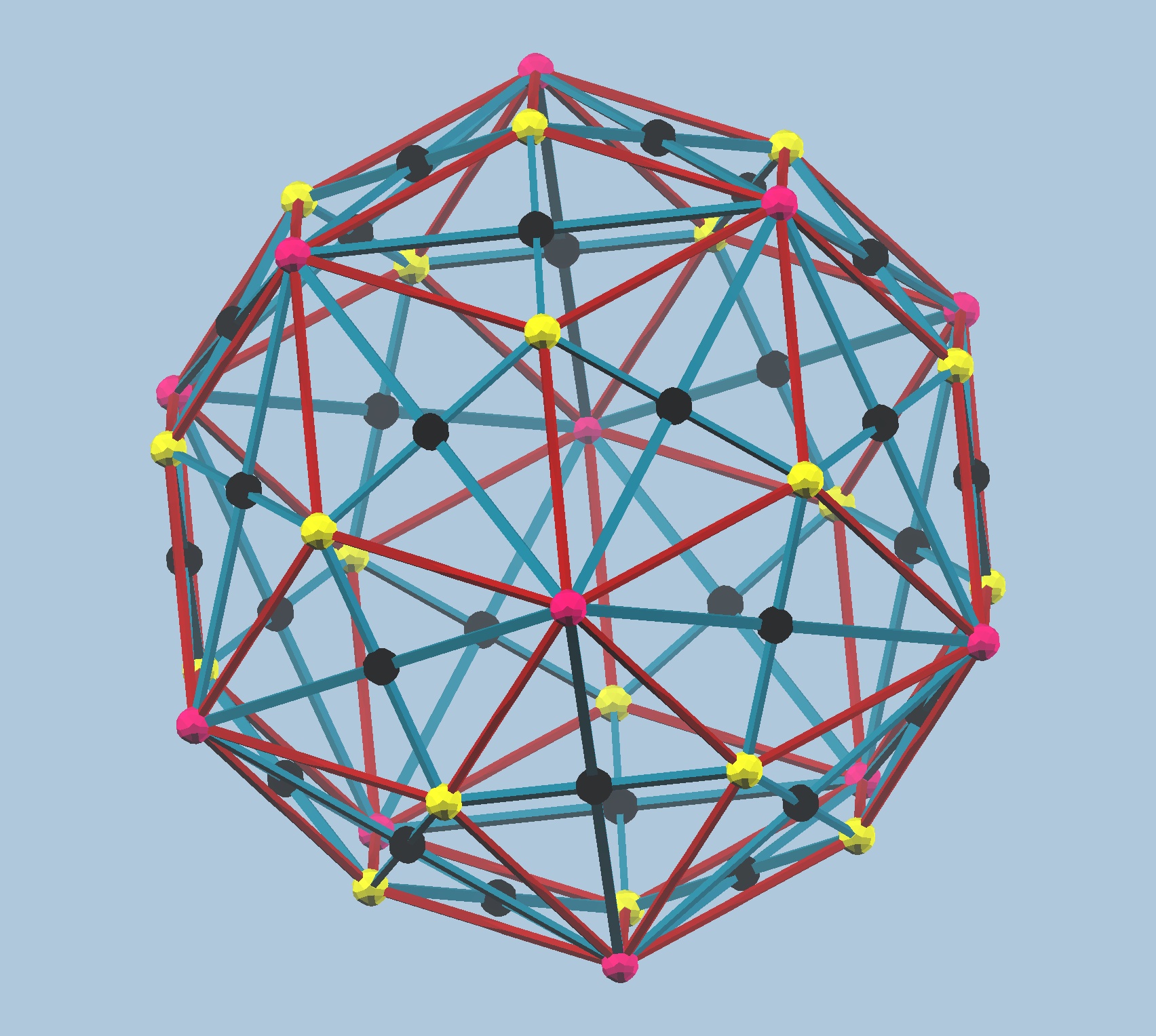
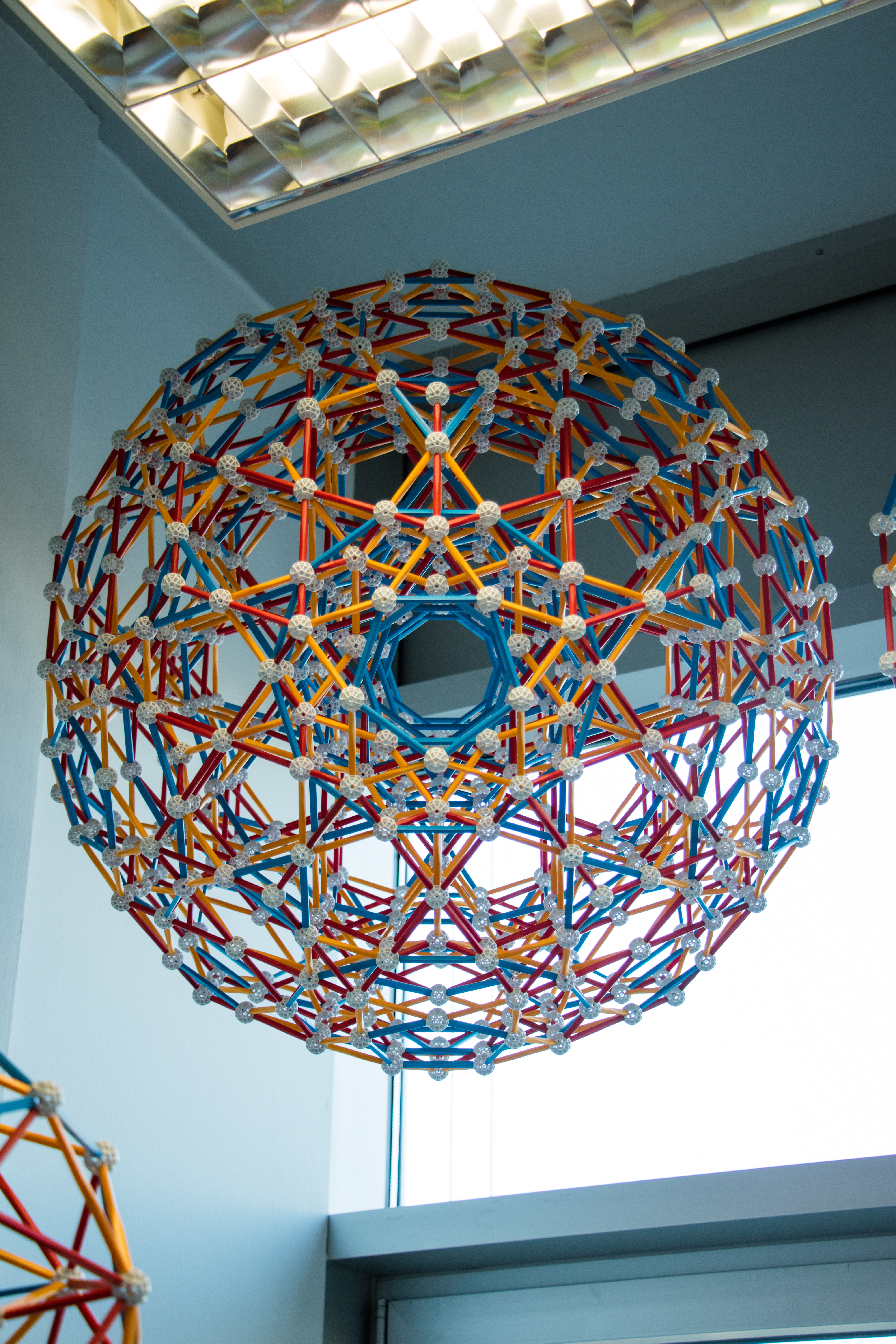
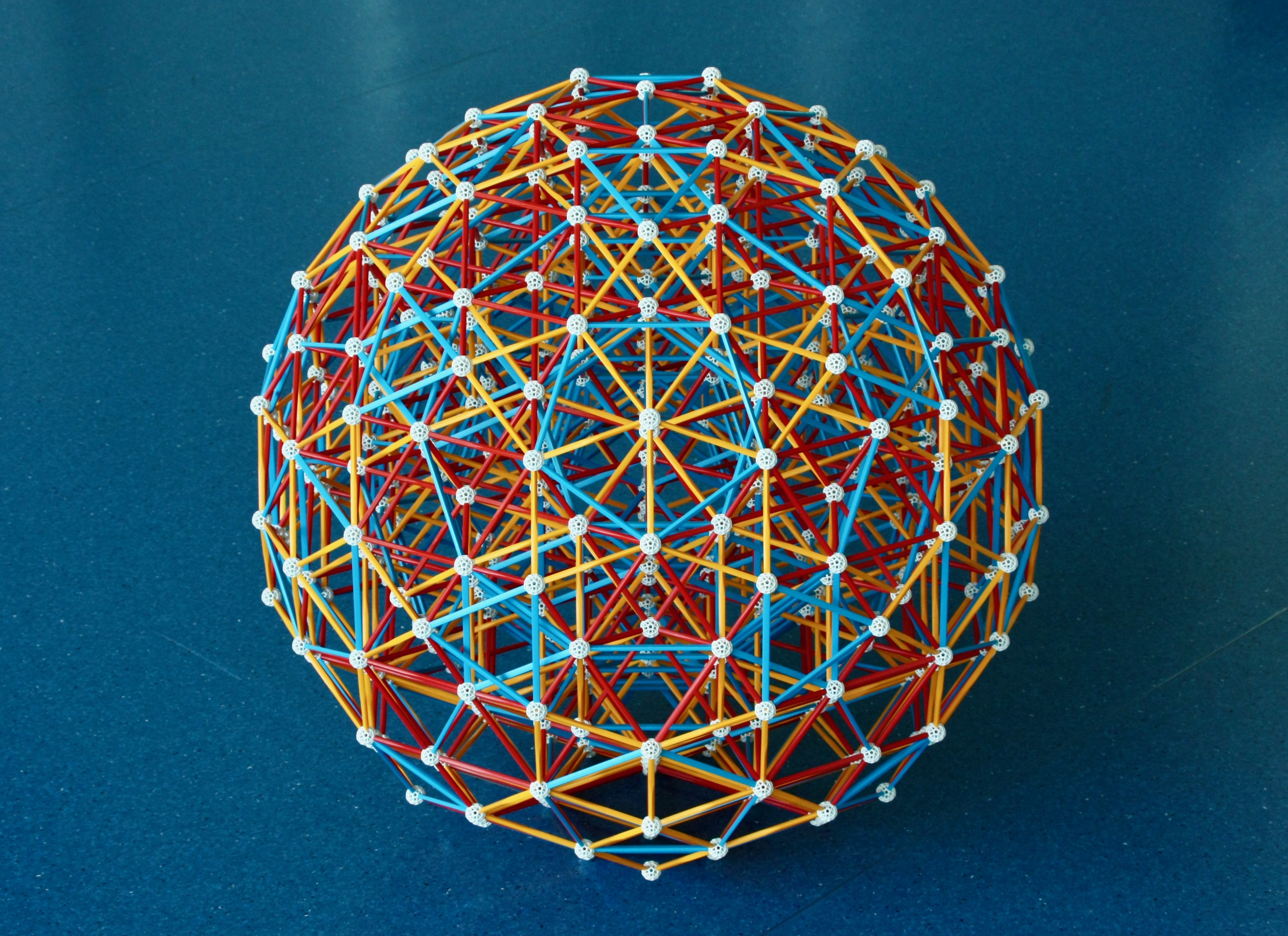
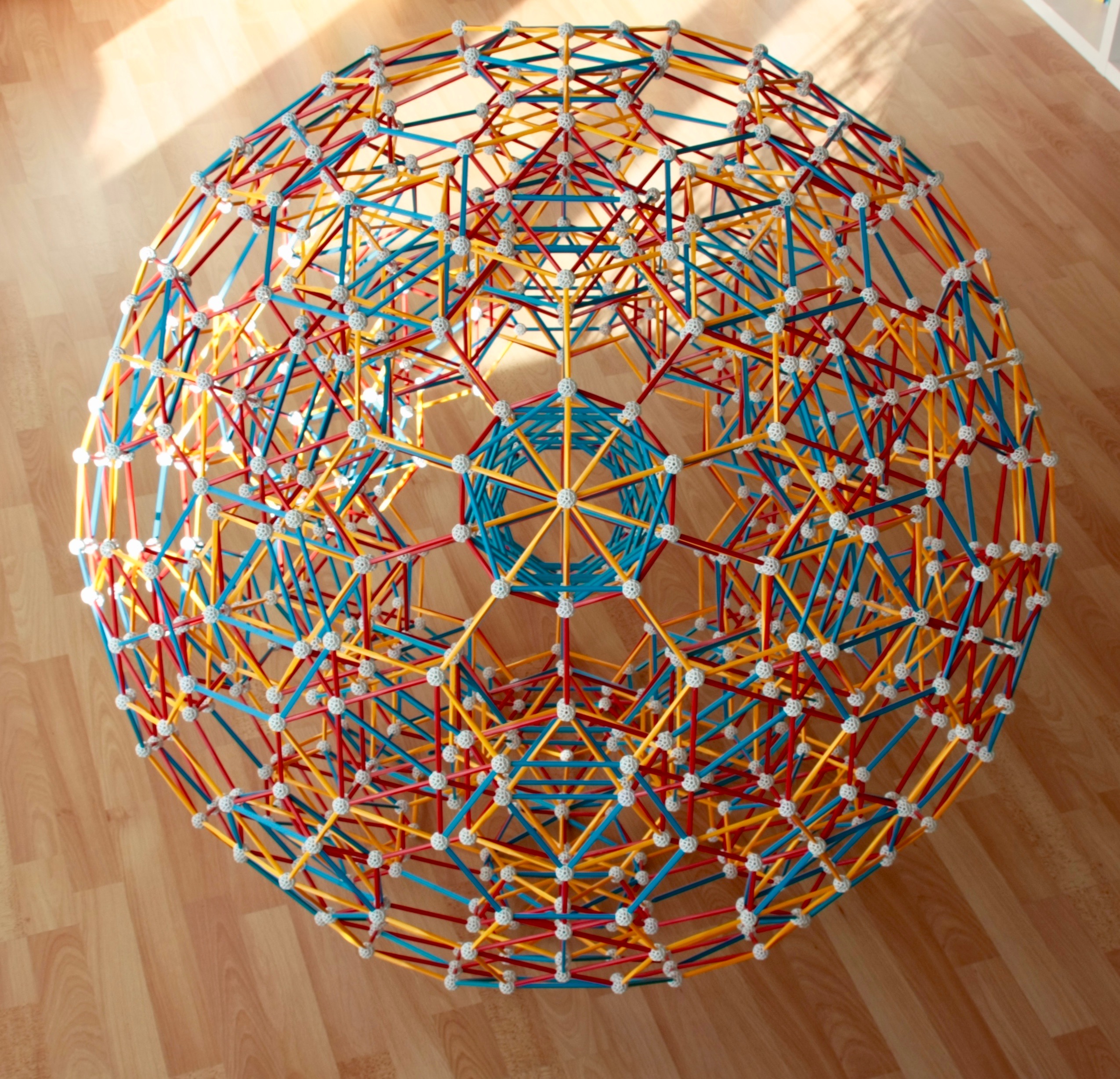
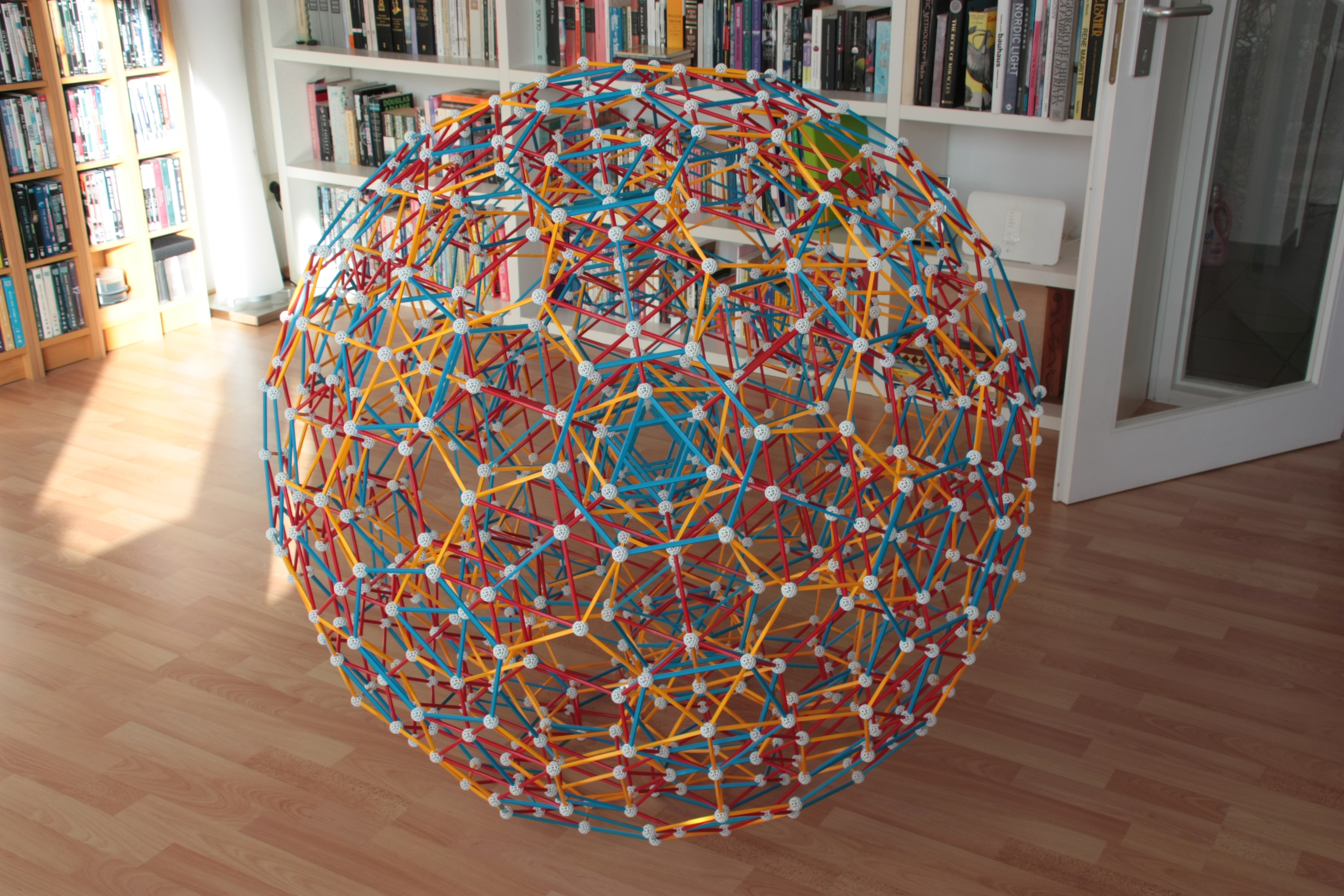
Fig. 9.4c: The icosahedral kaleidoscope. Note here how, using regular-sized B1 struts (for
the edges of the Dodecahedron) and B2 struts (for the edges of the Icosahedron, in yellow)
requires the use of two R1 struts to represent the edges of the Rombic triacontahedron
(see Figs. 2.2d, 4.9).
We now discuss several details of these figures:
I colour-coded the vertices according to the axis of k-fold symmetry where they are
located: red for the 5-fold symmetry (because those would connect to the centre with a R
strut), blue for 4-fold symmetry (because those would connect to the centre with a B
strut, although B struts have no 4-fold symmetry), Y for 3-fold symmetry (Y strut) and
black for 2-fold symmetry, for consistency with the models in Figs. 3.3a, b and c.
Whenever possible, I used HG and half-blue (HB) struts. This made the construction more
elegant, since I don't need to make all the edges of the Rhombic figures twice the length
of a Y or R strut (see Fig. 4.9). The disadvantage is that HB struts are exceedingly hard
to find, as they are no longer made by the Zometool company.
The requirement that both the edges of A and B appear in the figures does not complicate
them: in the case of the Tetrahedral and Icosahedral symmetries, each equatorial polygon
includes both the edges of A and B, as well as the edges of the rhombic polyhedra. For
detailed images of the equatorial polygons, see Figs. 9.5a, b and c.
All planes of bilateral symmetry intersect at the centre, around which the 3-D point
symmetry is defined. Outside that, they intersect along the axes of k-fold symmetry of
the polyhedron. Around these axes, any elements - and the whole polyhedron - have a k-fold
dihedral symmetry like that shown in Figs. 9.1a, b and c, 9.2a and b and Figs. 9.3a and b.
These planes divide a unit sphere around the central point into spherical triangles, known
as Möbius
triangles. They are the fundamental domains of the
respective point symmetry. They correspond to the triangles of the models in Figs. 9.4a, b
and c. Their angle at each vertex, which coincides with a k-fold symmetry axis, is 180
degrees/k, these numbers can be used to write them:
(2, 3, 3) triangles for the Tetrahedral symmetry, as we can see from Fig.
9.4a, 24 of these tesselate the sphere.
(2, 3, 4) triangles for the Octahedral symmetry, 48 tesselate the sphere (see
Fig. 9.4b).
(2, 3, 5) triangles for the Icosahedral symmetry, 120 tesselate the sphere
(see Fig. 9.4c).
In the case of all these triangles, the angles at the vertices add to more than 180
degrees. This is normal, these are spherical triangles. We should be aware that there
are, of course, other symmetries other than those of the regular polyhedra. As an example,
for a prism, we have instead: (p, 2, 2) triangles, where 2p triangles tesselate the
sphere. There is no limit for p.
One interesting feature of the kaleidoscope in Fig. 9.4c is the distribution of the white
connectors, which represent a slightly distorted version of the Rhombicosidodecahedron, an
Archimedean solid. Instead of Square faces around the axes of 2-fold symmetry, this
distorted version has Golden rectangles. Note how this represents the connectors
themselves, and how the orientation of the connectors is identical to the orientation of
the solid defined by the white connectors!
***
We've calculated the angles at the vertices of the Möbius triangles. We not calculate
the lengths of their edges. These are the angles, measured from the centre, between the
different axes of dihedral symmetry.
If we cut the models in Figs. 9.4a, b and c along their planes of bilateral symmetry, we
can see their equatorial polyhedra. Their vertices are connected to the center by the axes
of symmetry of the kaleidoscope, in these models we can see how they are arranged within
these planes; they show where the plane intersects other planes of bilateral symmetry. The
axes of symmetry are coloured like the balls they connect to, except for the axes of
2-fold symmetry: the balls are black, but the struts that connect to them (either by HG or
HB) are coloured teal.
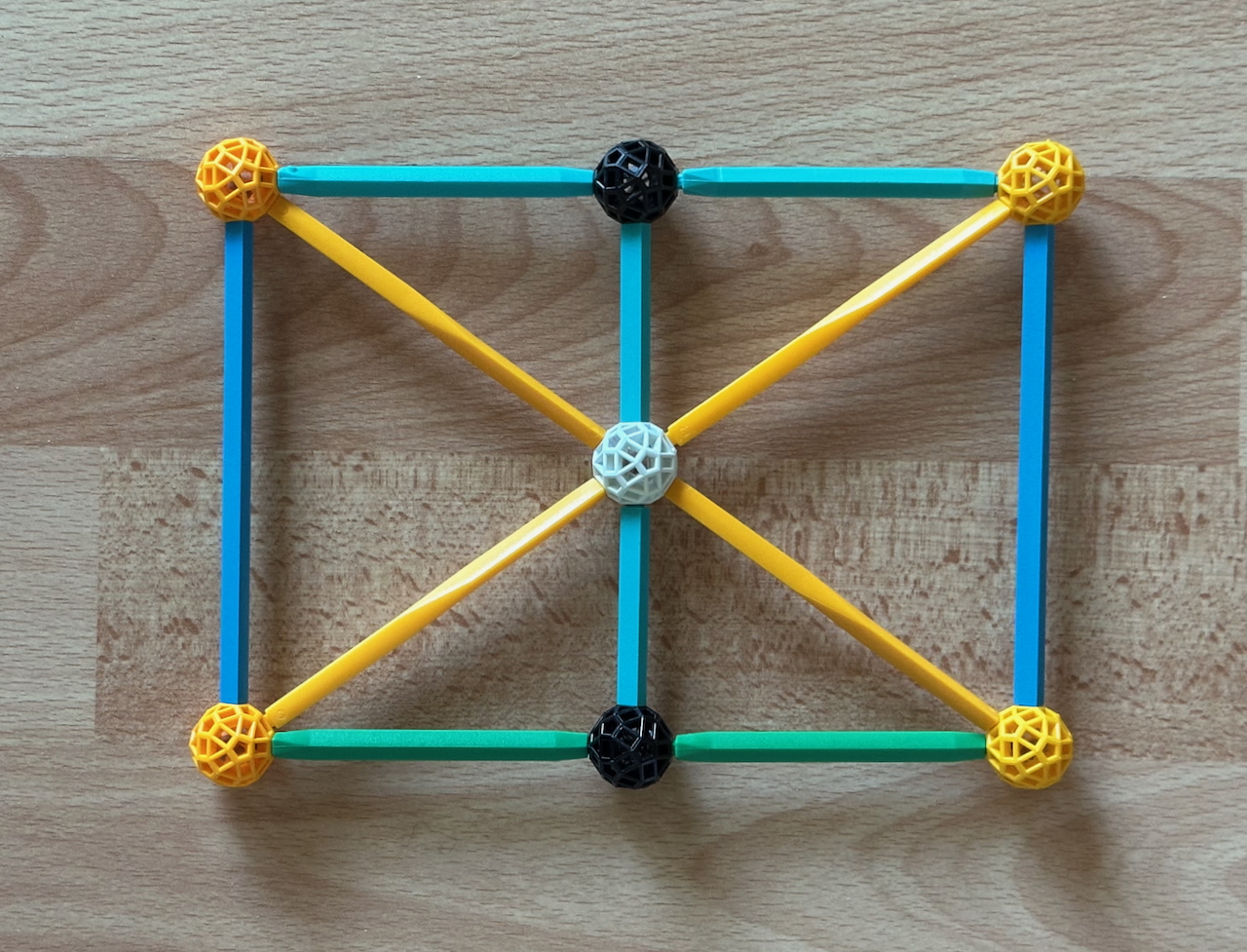
Fig. 9.5a: One of the six planes of bilateral symmetry of the Tetrahedral kaleidoscope.
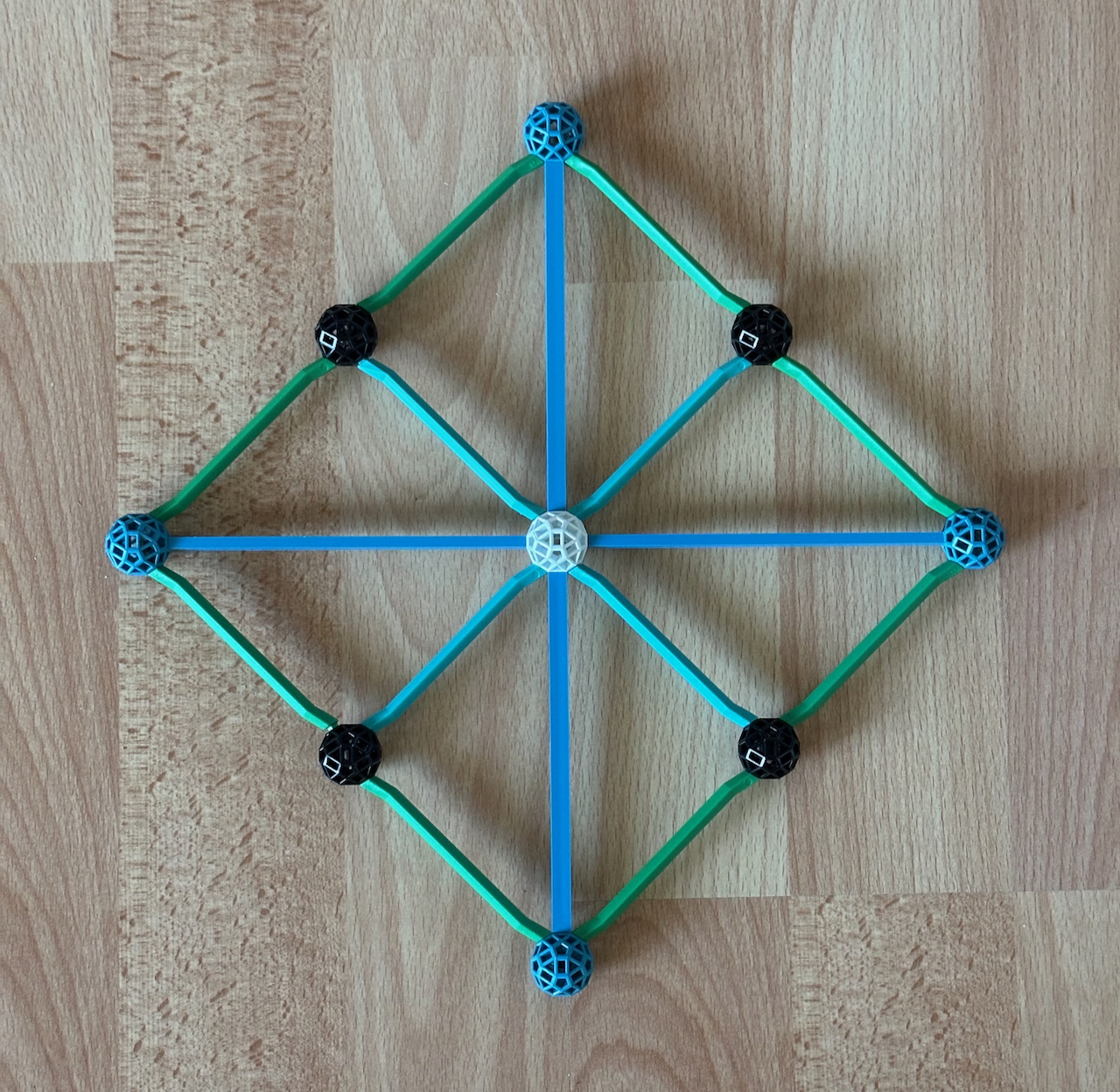
Fig. 9.5b: Three planes of bilateral symmetry of the Octahedral kaleidoscope have
4-fold symmetry; they contain the equatorial Squares of the Octahedra.
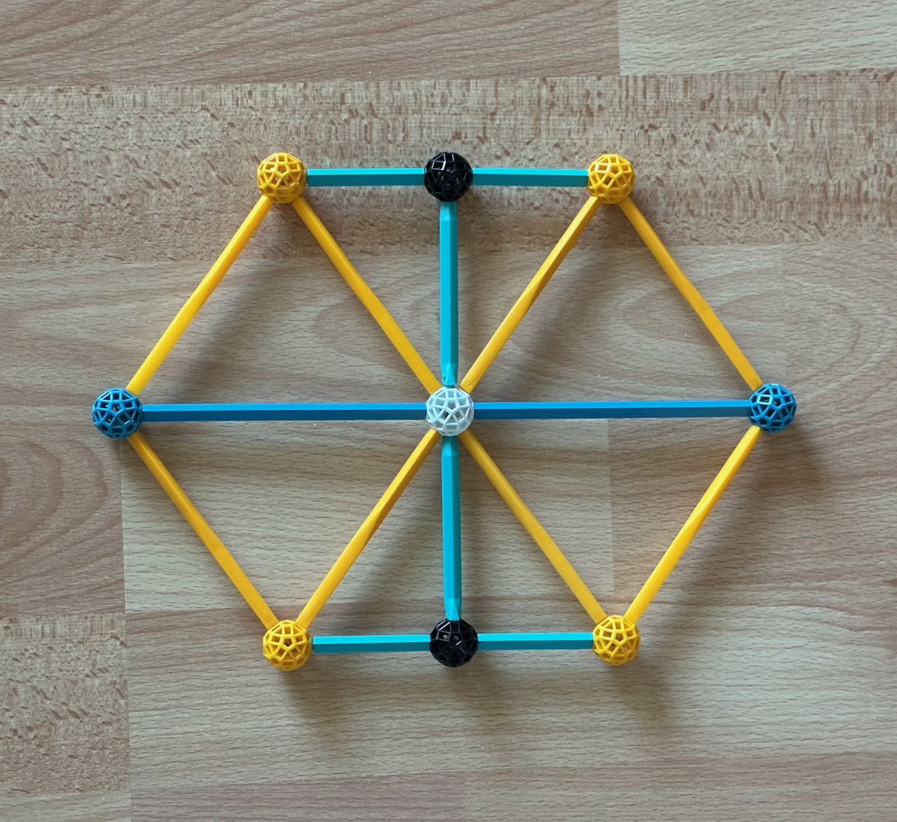
Fig. 9.5c: The six other planes of bilateral symmetry of the Octahedral kaleidoscope
are directly related to the six planes of bilateral symmetry of the Tetrahedral
kaleidoscope. They are very different from the three planes of symmetry in Fig. 9.5b.
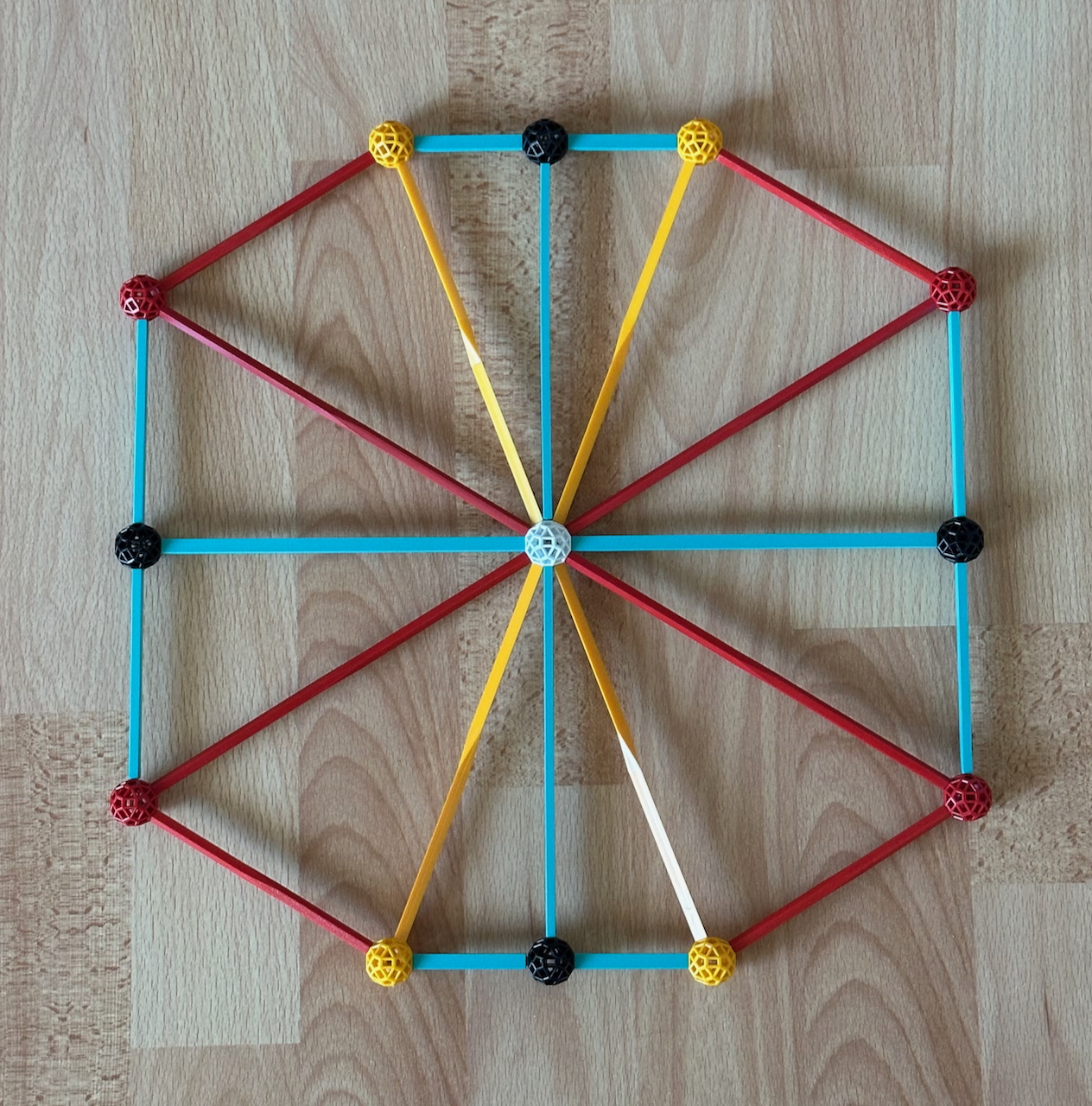
Fig. 9.5d: A plane of bilateral symmetry of the Icosahedral kaleidoscope. Note the
overall 2-fold symmetry, which has 2 axes of bilateral symmetry. As in the case of the
Tetrahedral kaleidoscope, all planes of bilateral symmetry are identical.
As discussed in the polyhedron page, the Tetrahedral kaleidoscope has four axes of 3-fold
symmetry, and three of 2-fold symmetry, neither with central symmetry. It has six planes
of bilateral symmetry, which go through opposite edges of the enveloping Cube. In Fig.
9.5a, note that the colours of the HG2 struts on top and below are different: the green
one represents an edge of the Tetrahedron, the other one doesn't. This emphasises the fact
that the Tetrahedral symmetry does not have central symmetry.
As discussed above, the Octahedral kaleidoscope has 3 axes of 4-fold symmetry, 4 axes of
3-fold symmetry and 6 axes of 2-fold symmetry. In Figs. 9.5b and c, we find an unusual
characteristic of this kaleidoscope, that it was two different types of planes of
bilateral symmetry. Three of these (Fig. 9.5b) have 4-fold symmetry; they contain the
edges of the Octahedron, which form equatorial Squares. Their 4-fold symmetry implies that
they are necessarily perpendicular to the 3 axes of 4-fold Octahedral symmetry. Six others
have 2-fold symmetry, they contain the edges of the Cube and of the Rhombic dodecahedron.
Their symmetry implies that they are necessarily perpendicular to the 6 axes of 2-fold
Octahedral symmetry. Because they include opposite edges of a Cube, they have the same
arrangement as the six planes of bilateral symmetry of the Tetrahedron.
As we've seen, the Icosahedral kaleidoscope has 6 axes of 5-fold symmetry, 10 axes of
3-fold symmetry and 15 axes of 2-fold symmetry. In Fig. 9.5d, we can see that its plane of
bilateral symmetry has itself an overall 2-fold symmetry, with 2 blue axes of bilateral
symmetry that are shared with the whole kaleidoscope. This symmetry implies these planes
are necessarily perpendicular to the 15 axes of 2-fold Icosahedral symmetry; there are
therefore 15 of these planes. We can check this by noting that each of the equatorial
polygons includes 4 of the 60 edges of the Rhombic triacontahedron, and 2 of the 30 edges
of the Icosahedron or Dodecahedron. From the symmetry of this figure, we can derive a
fundamental fact, that unlike the Tetrahedral symmetry, the Octahedral does not "fit"
within the Icosahedral symmetry. Indeed, in the Compound of five cubes, the arrangement of
vertices and edges above the faces of the Cubes is not invariant under a 90-degree
rotation; the same happens for the vertices of the Compound of five octahedra.
One of the advantages of these figures is that we can calculate very easily the angles
between the axes of symmetry as seen from the central point. We now go in detail through
these:
- In Fig. 9.5a, we see that the angle between the axes of 2-fold and 3-fold symmetry is
the angle between the diagonal and the short side of the Yellow rectangle (Fig. 2.2b),
this is arctan(√2) = 54.735 610 317 245... degrees. The angle between the two axes of
3-fold symmetry is 180 degrees minus twice the first angle, 70.528 779 365 509... degrees.
- In Fig. 9.5b, we see that the angle between the 2-fold and 4-fold symmetry axes of the
Octahedral kaleidoscope is 45 degrees. In Fig. 9.5c, we see that the angle between the
2-fold and 3-fold axes of symmetry is the angle between the diagonal and the long side of
the Yellow rectangle (Fig. 2.2b), this is arctan(1/√2) = 35.264 389 682 754...
degrees. The angle between the 3-fold and 4-fold symmetry axes is the complementary, i.e.,
the angle between the diagonal and the short side of the Yellow rectangle (Fig. 2.2b), 90
− 35.264 389 682 754... = 54.735 610 317 245... degrees, which we have met already
in the Tetrahedral kaleidoscope.
- In Fig. 9.5d, we see that the angle between the axes of 2-fold and 3-fold symmetry is
the angle between the diagonal and the long side of the Long yellow rectangle (Fig. 2.2e),
this is arctan(1/φ2) = 20.905 157 447 889 degrees. The angle between the
axes of 2-fold and 5-fold symmetry is the angle between the diagonal to the the long side
of the Golden rectangle (Fig. 2.2d), this is arctan(1/φ) = 31.717 474 411 461...
degrees. Finally, we see that the angle between the axes of 3-fold and 5-fold symmetry is
90 degrees minus the other two, 37.377 368 140 649... degrees.
These are thus the lengths of the edges of the spherical Möbius triangles. They add
to 180, 135 and 90 degrees in the cases of the Tetrahedral, Octahedral and Icosahedral
kaleidoscopes. They are all the information we need to build these kaleidoscopes. Detailed
instructions on how to do build paper models are provided by Wenninger (1974). Detailed
instructions on how to build actual working kaleidsocopes, with mirrors, are provided by
Coxeter (1991), chapter 3.
***
The kaleidoscopes associated with the symmetries of the regular polyhedra are now
completely defined. We can refer to its planes of bilateral symmetry as mirrors, since
they reflect each half of the polyhedron into another half. We now illustrate the Wythoff
construction using these Zometool models of their kaleidoscopes:
- Let's pick a vertex of the Tetrahedron in Fig. 9.4a. This is a yellow connector.
Because this vertex lies in the intersection of two mirrors of each triangle, its cannot
be reflected by those: the reflection would appear in the same point. To reflect that
vertex, the only neighbouring mirror sections available are those in teal (the edges of
the dual Tetrahedron); these reflect the vertex and edge to the positions of the
neighbouring vertices.
- Likewise, in Fig. 9.4b, we see that the vertices of the Octahedron (in blue) can only
be reflected by the teal mirror sections (the edges of the Cube). The vertices of the Cube
(in yellow) can only be reflected by the green mirror sections (the edges of the
Octahedron). The black vertices of the Cuboctahedron can only be reflected by the yellow
mirror sections (the edges of the Rhombic dodecahedron).
- And likewise in Fig. 9.4c: the vertices of the Icosahedron (in red) can only be
reflected by the edges of the Dodecahedron. The vertices of the Dodecahedron (in yellow)
can only be reflected by the edges of the Icosahedron. The black vertices of the
Icosidodecahedron can only be reflected by the red edges of the Rhombic
triacontahedron.
From this, it is clear that the regular polyhedra and their rectifications share the same
type of Wythoff construction: Their vertices are reflections of one of the three vertices
of the Möbius triangle (i.e., of points lying on the symmetry axes of the
kaleidoscope) by a single mirror, the one opposite to that vertex. Thus, in each case,
only one mirror is active. The fact that a triangle has only three vertices means that for
each pair of dual regular polyhedra (i.e., for each type of symmetry) there is only one
rectified form.
The main difference between two dual regular polyhedra and their rectification is the way
the edges are reflected. As we've seen in the derivation of the kaleidoscopes, the
edges of two dual regular polyhedra are necessarily in the planes of bilateral symmetry:
they coincide, respectively, with the two sides of the Möbius triangle that meet at a
right angle (at the black balls in Figs. 9.4a, b and c). Each such edge is shared by a
total of 4 such triangles, their number is therefore the number of Möbius triangles
in each symmetry / 4.
However, for the rectifications, this is not the case, as shown in Fig. 9.6.
Fig. 9.6: Icosahedral kaleidoscope, as in Fig. 9.4c, now with one edge of the
Icosidodecahedron (B2 strut in teal).
In this figure we start with the model of the Icosahedral kaleidoscope in Fig. 9.4c. As
we've seen above, the long side of the Möbius triangle is that of a Rhombic
polyhedron, in this case of a Rhombic triacontahedron. Here one of these sides
(highlighted by the black line) is reflecting one of the points of 2-fold symmetry, A,
into a second one, A'. Uniting A and A' is one of the edges of the Icosidodecahedron
(represented by a B2 strut in teal), which is therefore (as we've seen in the polyhedron
page) perpendicular to those of the Rhombic triacontahedron. This means that the edge of
the Icosidodecahedron does not coincide with any edge of the Möbius triangle and is
therefore within that triangle. In the Figure, we also see how the edge of the
Icosidodecahedron is shared equally by two Möbius triangles, as are the edges of the
Rhombic triacontahedron. This implies that their number is the number of Möbius
triangles in each symmetry / 2; i.e., twice the number of edges of the regular polyhedra.
We also see here that the way the edges of the rectifications are reflected by the two
perpendicular mirrors implies that there are four of them meeting at each of those black
balls. Therefore, they necessarily have a rectangular vertex figure, which as we've seen
in Fig. 9.1a, is a general product of the 2-fold symmetry around the black balls. As we've
seen already in the polyhedron page, the
central symmetry of these vertex figures implies that these rectifications have equatorial
Polygons.
One interesting fact, which we have already mentioned, is that the rectification of the
Tetrahedron is itself also regular, an Octahedron; its vertices are the black balls in
Fig. 9.4a, these are reflected by a single mirror, which in that figure is represented by
the edges of the Cube. Its edges are therefore perpendicular to those of the Cube, they
are the edges of the Octahedron. This highlights that, as for even-sided polygons (like
the Hexagon in Fig. 9.3b), some polyhedra can also have multiple Wythoff constructions.
This particular case of a multiple Wythoff construction will be of importance for what
follows.
There are other possible types of Wythoff construction for polyhedra, which are associated
with reflecting points located in the edges and inside the Möbius triangles. The
result of such constructions are the Archimedean solids.
***
A final question: can the regular star polyhedra be derived using the Wythoff
construction? The answer is yes, only that the Wythoff construction reflects vertices of
Schwarz
triangles, which have surfaces that are multiples (by a factor of d) of those of the
Möbius triangles. These cover the sphere d times as a multi-connected Riemann
surface. The number d is known as the density of the resulting
polytopes. The only two Schwarz triangles that yield regular polyhedra (the Kepler-Poinsot
polyhedra) are:
(2, 5/2, 5) - these have d = 3; they generate the Stellated dodecahedron and the Great
dodecahedron.
(2, 5/2, 3) - these have d = 7; they generate the Great icosahedron and the Great
stellated dodecahedron.
Because they have a right angle (the "2" at the start), they also generate the
rectifications of these polyhedra, respectively the Dodecadodecahedron and the Great
icosidodecahedron, which have similar properties to the rectifications mentioned above.
There are many other Schwarz triangles, which generate all but one of the 75 non-prismatic
uniform star polyhedra, the "Star
archimedeans".
However, there are cases where multiples of the smaller Möbius triangles fit into
larger Möbius triangles. This is the origin of the regular compounds: as the
Wythoff construction starts reflecting the vertices of these triangles, it will only
generate the vertices of the regular polyhedra with the symmetry associated with those
triangles. Two Möbius triangles of the Octahedral group fit inside a Möbius
triangle of the Tetrahedral group (their numbers are 48 and 24 respectively) this gives
rise, via the Wythoff construction, to the Stella Octangula, which has d = 2. Five
Möbius triangles of the Icosahedral group fit inside a Möbius triangle of the
Tetrahedral group (their numbers are 120 and 24 respectively); this gives rise to the
regular compounds with Icosahedral symmetry, which have d = 5 or 10.
***
Just like we can apply the concept of the Wythoff construction to polyhedra, we can also
apply it to the regular tilings of 2-D Euclidean space, which are no longer point
symmetry groups, but flat analogs of the polyhedral surface. Doing this, we obtain all the
Archimedean tilings of 2-D Euclidean
space, with the exception of the elongated triangular
tiling, which is non-Wythoffian. These tilings are of practical interest for fields
like architecture, design and engineering.
The Wythoff construction in 4D
The Wythoff construction works in analogously in any dimensional space. We will now
discuss in particular how things work in 4 dimensions.
To build the kaleidoscope, we must first have a central point, from where the 4-D
point symmetry is defined. Intersecting at this point are "hyperplanes" of bilateral
symmetry. These 3-D "planes" intersect a 3-sphere centred on that point along
particular 2-D surfaces of bilateral symmetry. These divide the 3-sphere into Goursat
tetrahedra, the fundamental domains of these 4-D point symmetries.
The vertices of these tetrahedra, where three 2-D surfaces meet, correspond to the
intersections of the 3-Sphere with axes of polyhedral symmetry - as we've seen,
projecting the polychoron along these axes we obtain projections with the respective
symmetry. If a cell of a polychoron is centered on such a vertex, or a vertex coincides
with it, those cells or vertex figures will have the same polyhedral symmetry. The edges
of these tetrahedra, where two 2-D surfaces meet, correspond to the axes of k-fold
dihedral symmetry we've seen for polyhedra; if an edge of the polychoron is coincident
with one of those, its edge figure is a k-sided polygon, if a face is perpendicular to
them, it is a k-sided polygon as well. The faces of these tetrahedra are in the 2-D
surfaces, so like them they are are associated with bilateral symmetry. This means that if
the faces of a polychoron coincide with these, they must separate identical cells, if an
edge is bisected by them, it must link identical vertices.
For two dual regular polychora A and B, two of the vertices of polyhedral symmetry of the
Goursat tetrahedron correspond to the centres of cells and vertex figures of A, which by
duality correspond to the vertex figures and cells of B, with the same symmetries. By
definition, the polyhedral symmetries associated with the cells and vertices must be those
of regular polyhedra. What about the other two vertices? These can be found easily from
the fact that each edge of A goes through the centre of a face of B, and vice-versa, this
implies that each edge and each face of regular polychora A and B must be associated, at
the same time, with bilateral and dihedral symmetry. Thus, their central points correspond
to axes of polyhedral symmetry that combine dihedral and bilateral symmetry: the prismatic
symmetries.
The vertices of two dual regular polychora A and B are built by reflecting the two
vertices of the Goursat tetrahedron associated with regular polyhedral symmetries. As for
the polyhedra, the rectifications of regular polychora also share the same type of Wythoff
construction: reflecting vertices of the Goursat tetrahedron, only this time those
associated with prismatic symmetries. They have two types of cells, which are associated
with the two axes of regular polyhedral symmetry.
***
We now exemplify all of this with a more detailed discussion of the Hexacosichoric
symmetry and its kaleidoscope. Reflecting the vertices on the 60 axes of Icosahedral
symmetry we obtain the vertices of the 600-cell (Fig. 5.10), reflecting the vertices on
the 300 axes of Tetrahedral symmetry we obtain the vertices of the 120-cell (Fig. 5.11).
In the next two Figures, we show their rectifications, which share their Hexacosichoric
symmetry. We see clearly in both models how their vertices (which appear in the middles of
the edges of the polychora they rectify) are associated with the prismatic symmetries
associated with the edges and faces of the 120-cell and 600-cell: their vertex figures are
a Triangular prism in the case of the 1200 vertices of the Rectified 120-cell in Fig. 9.7
and a Pentagonal prism in the case of the 720 vertices of the Rectified 600-cell in Fig.
9.8. Both have two sets of cells, one with Icosahedral and a second one with Tetrahedral
symmetry, the Octahedral cells of the Rectified 600-cell are rectified Tetrahedra.
These vertices are reflections of the points associated with the Triangular and Pentagonal
prismatic symmetries of the Goursat tetrahedra, they mark the position and number such
points in the Hexacosichoric kaleidoscope. They imply that, in addition to the
aforementioned axes of Icosahedral and Tetrahedral symmetry, this kaleidoscope has 600
axes of Triangular prismatic symmetry and 360 axes of Pentagonal prismatic symmetry. The
intersections of these axes with the unit 3-sphere are the vertices of Goursat tetrahedra
of the Hexacosichoric kaleidoscope.
Fig. 9.7: The icosidodecahedral cell-first projection of the Rectified 120-cell.
How to build: Study the perspective-flattened Dodecahedra in the model of the
120-cell. Make models of Icosidodecahedra with similar flattening. Then have a look at the
Eusebeia page on the
Rectified 120 cell.
Picture taken by Jason Wu.
In the Icosahedral projection of the rectified 120-cell, the Dodecahedra of the 120-cell
are replaced by their rectifications, Icosidodecahedra. Under each of the 600 vertices of
the 120-cell, a Tetrahedron (the vertex figure of the 120-cell) appeared. Three
Icosidodecahedra and two tetrahedra meet at each vertex. Each edge is shared by a
Tetrahedron and two Icosidodecahedra. This Icosahedral projection is necessarily centred
on an Icosidodecahedral cell.
In the page on the regular convex polychora,
we have seen two semi-regular convex
polychora (which, apart from being Uniform, have only regular cells, in these cases of
two distinct types): the Rectified 5-cell and the Snub 24-cell. There is a third and last
semi-regular convex polychoron, the Rectified 600-cell. Like the Rectified 5-cell, this
results from rectifying a regular convex polychoron with Tetrahedral cells: the 600
Tetrahedra of the 600-cell are replaced by their regular rectifications, Octahedra. Under
each of the 120 vertices of the 600-cell new Icosahedra (the vertex polyhedron of the
600-cell) appeared; all their projections were already visible in the model of the
600-cell in Fig. 5.10. Three Icosahedra and five Octahedra meet at each vertex; each edge
is shared by one Icosahedron and two Octahedra.
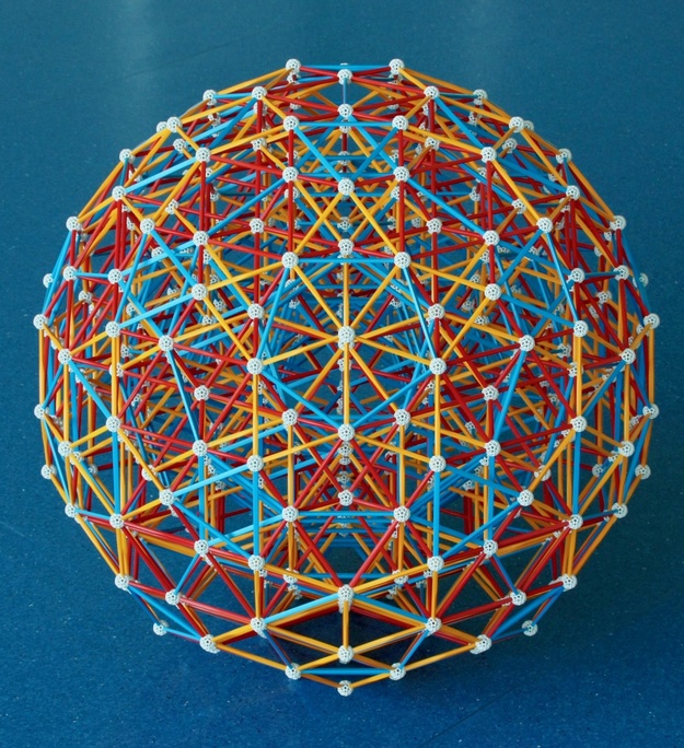
Fig. 9.8: The Icosahedral projection of the Rectified 600-cell. This projection is
the rectification of the Icosahedral projection of the 600-cell.
How to build: After studying the perspective-flattened Icosahedra in the model of
the 600-cell, have a look at the Eusebeia page on the Rectified 600 cell.
Also recommended is David Richter's page on
the Rectified 600-cell.
Also, as for the other semi-regular polychora, all faces are Triangular. Since all faces
are Triangular, the prismatic vertex figures are necessarily edge sections located under
each vertex, as in the case of the Rectified 5-cell and Rectified 16-cell (the 24-cell).
If you pay close attention to the model, you will be able to see several Archimedean
solids in blue, starting with Icosidodecahedra - the rectifications of the Icosahedral
sections of the 600-cell. These polyhedra are also edge sections of the Rectified
600-cell. Because they have Icosahedral symmetry, they appear ``under'' the Icosahedral
cells in 4-D space, around the central cells in this projection. Studying the model
further, you will be able to see many flattened versions of those. All these edge sections
are the cells of 14 non-convex edge facetings of the Rectified 600-cell, all represented
by the same model. One of them is the Rectified icosahedral 120-cell, which has Great
dodecahedra and Icosidodecahedra as cells (for more about the Icosahedral 120-cell, see
the page on regular star polychora).
These 14 edge-facetings are a sub-group of the 60 facetings of the Rectified 600-cell
that are uniform, non-convex polychora.
In these models, we can see a general feature of these rectifications: the prismatic
symmetries around their vertices have no central symmetry. This means that there are no
equatorial polyhedra associated with them, which is unlike what we find for most of the
regular polychora. The situation is almost the reverse of what we find among regular
polyhedra, where only one of the nine regular polyhedra (the Octahedron) has equatorial
polygons, but all their rectifications (which the Octahedron also is) have, by virture of
their rectangular vertex figures, equatorial polygons. On the other hand, the
Icosidodecahedral cells of the Rectified 120-cell and all cells of the Rectified 600-cell
have central symmetry. This means that we can see equatorial cell rings. Some of these are
visible along the 5-fold symmetry axes of the Rectified 120-cell (we see one of these at
the centre of Fig. 9.7), because the Icosidodecahedra connect to each other at common
Pentagonal faces. For the Rectified 600-cell, equatorial cell rings are visible along the
3-fold symmetry axes, and they include alternate Icosahedra and Octahedral pairs, which
connect with each other at their common Triangular faces.
There are other possible types of Wythoff construction for convex polychora, which are
associated with reflecting points located in the edges, faces and inside the Goursat
tetrahedra.
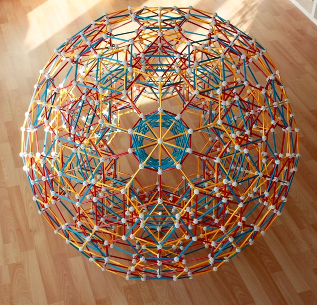
Fig. 9.9a: The Truncated 600-cell, here seen along one of its 5-fold symmetry axes.
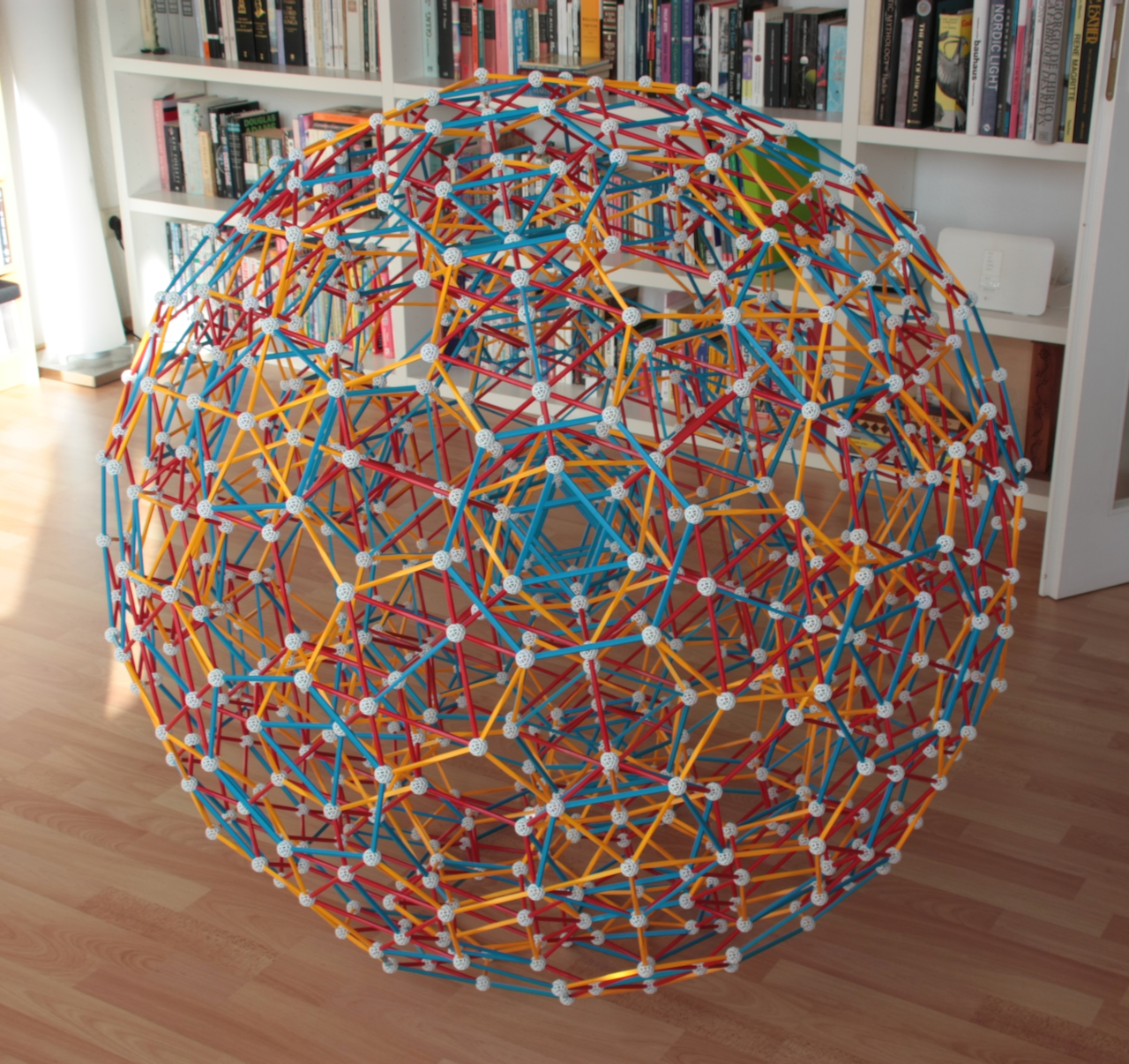
Fig. 9.9b: The same model as above, seen here from a 3-fold symmetry axis.
How to Build: See the Eusebeia page on the Truncated 600-cell
A reflection of a point in an edge of the Goursat tetrahedron results in the vertices of a
truncation. In Figs. 9.9a, b, we see the Icosahedral projection of the Truncated
600-cell. It is similar to the Rectified 600-cell above, and it also has 120
Icosahedral cells. However, instead of 600 Octahedral cells, it has 600 Truncated
tetrahedral cells. In Fig. 9.9b, we see the model along a cell ring that lies along one of
is axes of 3-fold symmetry. Along this axis, two Truncated tetrahedra connect to each
other via common Hexagonal faces, and to Icosahedra via common Triangular faces.
The rectifications discussed above, the Snub 24-cell and the Truncated 600-cell are
examples of Archimedean polychora; these are discussed in more detail here.
***
Just like we can apply the concept of the Wythoff construction to polychoral
kaleidoscopes, we can also apply it to Goursat tetrahedra that fill 3-D Euclidean space.
In these cases, we are no longer dealing with the type of kaleidoscope associated with
finite point-symmetry groups. Doing this, we obtain most of the uniform honeycombs, the
flat analogues of uniform polychoral surfaces, one of these, the Cubic honeycomb, is regular.
However, some such uniform tilings are non-Wythoffian.
These honeycombs are of practical interest for fields like architecture, design,
engineering and crystallography.
Coxeter-Dynkin diagrams
To proceed, we will now investigate in some detail the concept of a Coxeter-Dynkin diagram
(henceforth CD diagrams). These are graphs that describe
the fundamental regions of the kaleidoscopes we have seen above and the polytopes built
from them in an extremely compact and elegant way.
For dihedral symmetries, like the 2-fold (Figs. 9.1a, b and c) and 3-fold symmetry (Figs.
9.2a and b and 9.3a and b), the graph consists of two dots with line between them. The two
dots represent the two mirrors that define the border of the fundamental region. The line
indicates the dihedral symmetry of the kaleidoscope, i.e., the angle between the mirrors.
Below, we represent these graphs (how else?) with the Zometool: the dots are connectors,
the lines are struts. The graphs have the following rules: for a 2-fold symmetry, the line
is invisible, i.e., there is no strut! The 3-fold symmetry is indicated by an unmarked
line (in the Zometool version, a yellow strut). For 4 and 5-fold symmetries, the lines
have a number above them indicating the dihedral symmetry; in the Zometool version we will
indicate these with blue or red struts, as these represented these symmetries in the
corresponding vertices in the models of the kaleidoscopes in Figs. 9.4a, b and c and 9.5a,
b, c and d.
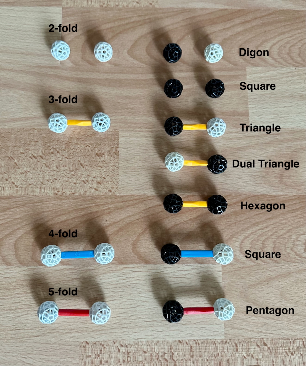
Fig. 9.10: CD graphs for dihedral kaleidoscopes (left), and for the polygons built with
them (on the right).
The graphs described above represent only the kaleidoscope. To represent a polytope, the
nodes are ringed, indicating which mirrors of the fundamental region are active during the
Wythoff construction. In the Zometool version, we represent ringing by turning a connector
black. Ringing a single node indicates that only one mirror is active, this means that the
point being reflected is located in the other mirror (Figs. 9.1b, 9.2b). Doing this, we
obtain a Polygon with the same number of sides as the symmetry. Ringing the other node
means that the other mirror is the one that is active, in this case we obtain the dual
Polygon (red Triangle in Fig. 9.3a). Ringing both nodes indicates that both mirrors are
active, i.e., the point is in the middle of the fundamental region: we then obtain a
polygon with twice the number of sides (the Square in Fig. 9.1c and the Hexagon in Fig.
9.3b). Note that the Square is also obtained by ringing a single node of the graph
associated with the 4-fold dihedral symmetry, this is a reflection of the aforementioned
fact that the same polytope can result from different Wythoff constructions acting on
different kaleidoscopes.
***
For 3-D symmetries, the CD graphs have three nodes and three lines connecting them. The
lines correspond to the vertices of the Möbius triangles, and list the dihedral
symmetries associated with each vertex, following the same rules as in Fig. 9.10. One of
the consequences (at least for the polyhedral kaleidoscopes we studied above) is that one
of the lines is invisible, the line corresponding to 2-fold symmetry. This is the reason
why these graphs are represented by lines, instead of having the triangular shapes they
depict. Not all kaleidoscopes have a single invisible line: the prismatic symmetries
include two empty lines, some other symmetries have no invisible lines.
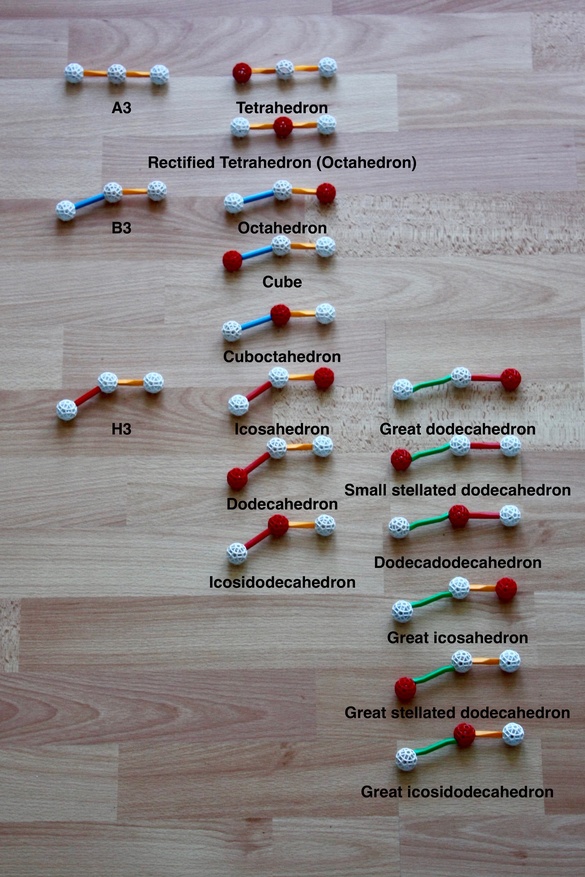
Fig. 9.11: CD graphs for polyhedral kaleidoscopes (left), and for the polyhedra built
with them (right).
As above, the nodes represent the edges of the Möbius triangles, the mirrors of the
kaleidoscope. Ringing a node indicates its mirror is active during the Wythoff
construction. Again, ringing a single node means that only one mirror is active, i.e.,
the point being reflected is at the intersection of the other two mirrors, i.e., in one of
the vertices of the Möbius triangle.
Ringing one end node of the graph represents, in the symmetries in Fig. 9.11, the
construction of a regular polyhedron. Ringing the node at the opposite end of the graph
produces the dual regular polyhedron. If the CD graph is symmetric (which it is for the
Tetrahedral symmetry), then the regular polyhedra obtained from ringing either end are
identical (Tetrahedra), this means that the tetrahedron is self-dual. Ringing the middle
node produces the rectification of the regular polyhedra. Importantly, note the two graphs
for the Octahedron, which can be obtained by ringing an end node in the Octahedral
symmetry, and the middle node in the Tetrahedral symmetry. This represents two different
Wythoff constructions of this polyhedron.
These graphs are very instructive. Cutting a note at the end opposite to the one being
ringed we see the faces of the polyhedron, in the example at the bottom we do this for the
Dodecahedron, revealing a Pentagon. Cutting the ringed node, and ringing the one closer to
it, we see the vertex figure, when we do this to the Dodecahedron, we see a Triangle. For
the rectified polyhedron, we see that both polygons are faces, as both touch the node
being ringed.
***
For 4-D symmetries, the CD graphs extend those in Fig. 9.11, they now represent the
four polyhedral symmetries associated with the Goursat tetrahedron.
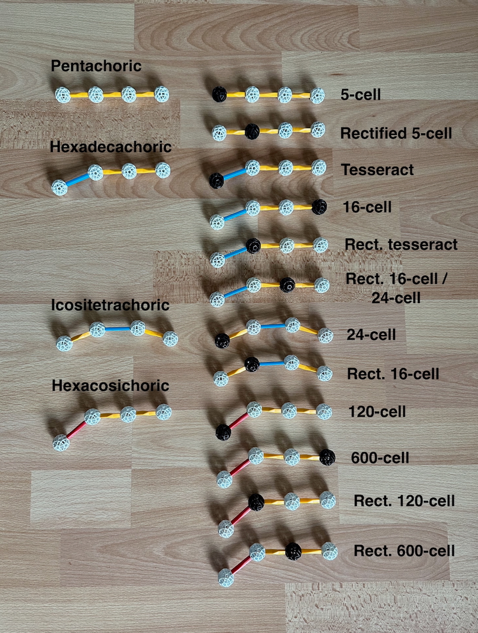
Fig. 9.12a: CD graphs for polychoral kaleidoscopes (on the left), and for the regular
polychora and their rectifications built with them (on the right).
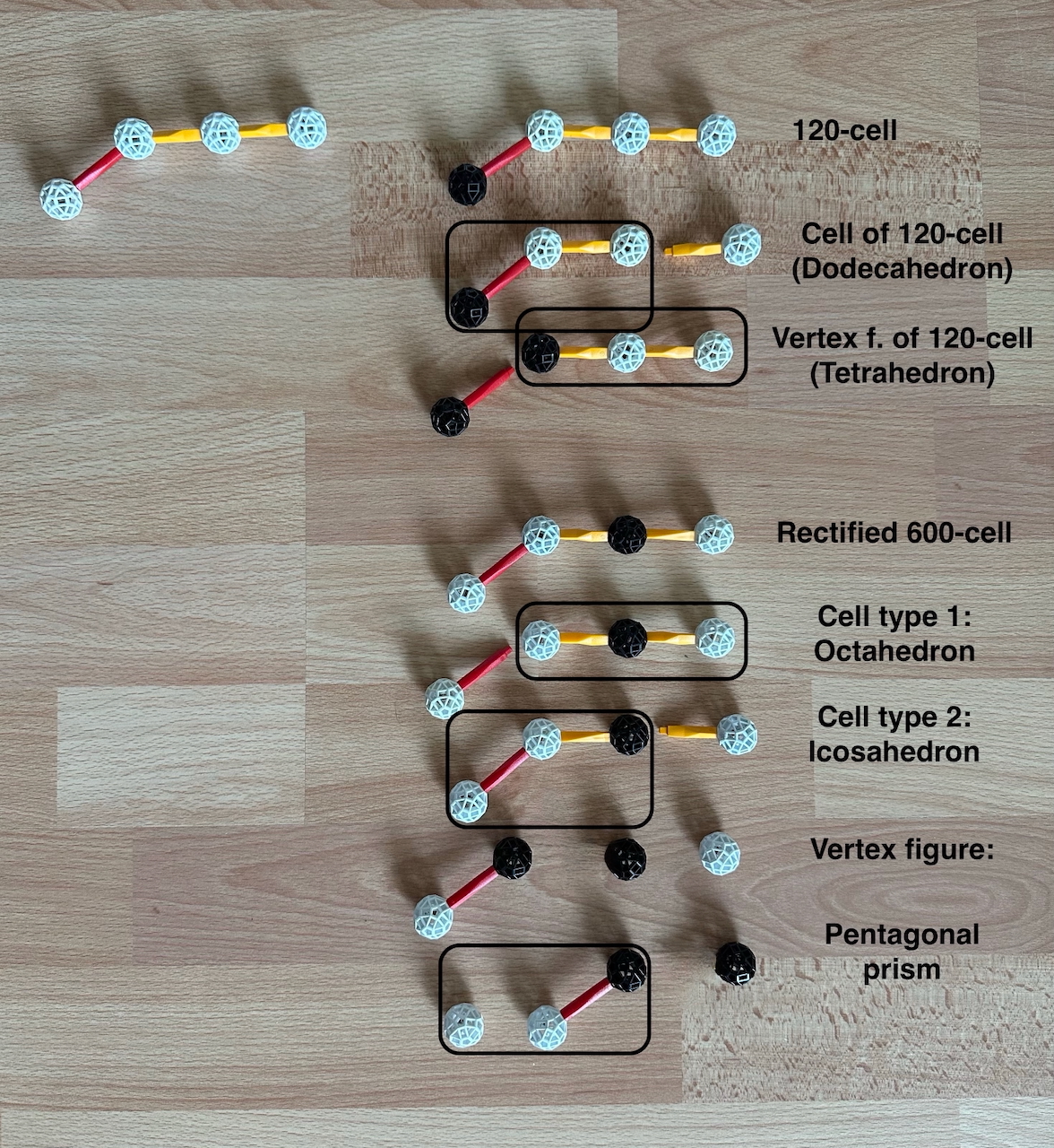
Fig. 9.12b: Example with how to read the cells and vertex figures for the 120-cell and
rectified 120-cell.
As before, ringing a single node means that only one mirror is active, i.e., the point
being reflected is at the intersection of three other mirrors, which means at one vertex
of the Goursat tetrahedron.
Ringing either of the end nodes of the graph represents, in the symmetries in Fig. 9.12a,
the construction of two dual regular polychora. For each regular polychoron, we see that
the lines in the graph represent the dihedral symmetries of the faces, the vertex figure
of the cells and the edge figures. If the CD graph is symmetric (which it is for the
Pentachoric and Icositetrachoric symmetries), then the regular polychora obtained from
ringing either end are identical (5-cells and 24-cells respectively), this means that they
are self-dual. Ringing the middle nodes corresponds to the rectifications. For symmetric
graphs the two rectifications are also identical to each other - however, they are
not self-dual. Note the two graphs for the 24-cell: this can be obtained as the
Rectified 16-cell and also by ringing the kaleidoscope associated with its "native"
Icositetrachoric symmetry at one end. This symmetry has no analogue in any other
dimensional space.
In Fig. 9.12b, we show how cutting a note at the end opposite to the one being ringed we
see the cells of the polychoron: doing this for the CD graph of the 120-cell, we obtain
the CD graph of the Dodecahedron. Cutting the ringed node, and ringing the one closer to
it, we see the vertex figure; doing this for the 120-cell we obtain the Tetrahedron. For
the rectified polychora, we see that there are two types of cells. In the example in Fig.
9.12b, we see that removing alternate nodes of the CD graph of the Rectified 600-cell we
obtain the CD graphs of Octahedra (as a rectified Tetrahedron) and Icosahedra. Cutting
the ringed node and ringing the next node - in either direction - we see that the vertex
figure is a Pentagonal prism (note the similarity with the top CD graph in Fig. 9.11);
to do this we need to keep in mind that the two end nodes are linked by an invisible line
denoting the 2-fold symmetry. In the last line, we merely rotated the CD graph of the
Rectified 600-cell by one node.
***
We now come to a new type of CD graph, one with three branches. This is the graph for
the demi-tesseractic symmetry. In Fig. 9.13, we see how this can be derived from the
demicubic symmetry of the Tetrahedron.
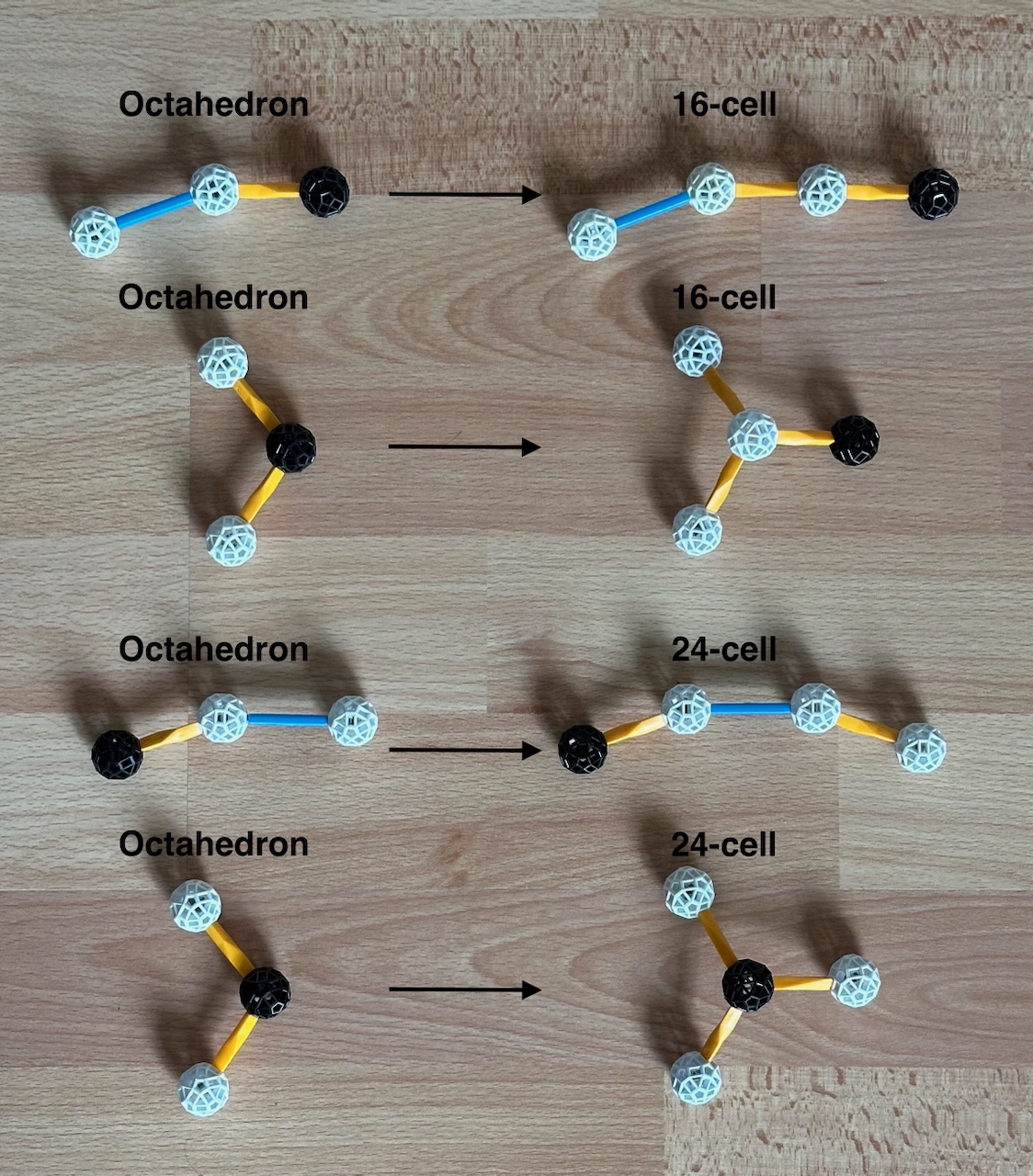
Fig. 9.13: CD graphs for Octahedra and its relatives in four dimensions. The
transformations are indicated by the arrows.
At the top, we transform the Octahedron into a 16-cell by adding another node, linking it
with a strut with 3-fold symmetry, and ringing the new node instead. Doing this, we obtain
the 16-cell. Whenever we add a new node and change the ringing to it, the preceding
polytope is the vertex figure of the new one, this means that the Octahedron is the vertex
figure of the 16-cell.
Next, we do the same to the Octahedron, but now represent it as a Rectified tetrahedron.
Adding one node and strut, we must obtain, again, the 16-cell. Note that, although the
polychoron is the same, the underlying symmetry used to build it in this second case
(demitesseractic) is not identical to the one used on top (hexadecachoric): as discussed
in detail here, the
latter can generate uniform polychora with Octagons, because it has a 4-fold strut in its
CD graph (as mentioned in Figs. 9.1c and 9.3b, and also 9.10, double ringing leads to a
polygon with twice the symmetry); the demitesseractic symmetry has no 4-fold symmetries.
In the third row, we start again with the Octahedron, and add a node at the opposite end
instead. It is clear that the Octahedron will be a cell of the new polychoron. A
comparison with Fig. 9.12a will show at once that the new polytope is, of course, the
24-cell (it is the only regular polychoron with Octahedral cells), built with its "native"
Icositetrachoric symmetry.
In the last row, we do the same, but again with the CD graph of the Octahedron as a
Rectified tetrahedron. The result is again the 24-cell, but this time built as a Rectified
demitesseract. As we saw in the first and second rows, the demitesseract is the 16-cell,
and as mentioned above, the 24-cell is a rectified 16-cell.
***
What is the geometric meaning of the three-fold CD graphs? In the linear CD graphs,
ringing a node at either end produces two dual polychora. This duality stems from the fact
that the extreme nodes are linked by an invisible 2-fold strut, which indicates a right
angle. The edges of two dual polyhedra are perpendicular to each other; the edges and
faces of two dual regular polychora are also perpendicular to each other.
In the CD graph of the demitesseractic symmetry, the same is happening, only that this
time is the three outer nodes that are connected to each other with three invisible 2-fold
struts. This means that the Goursat tetrahedron has three right angles, which are apparent
at the centre of a model of this tetrahedron in Fig. 9.14.
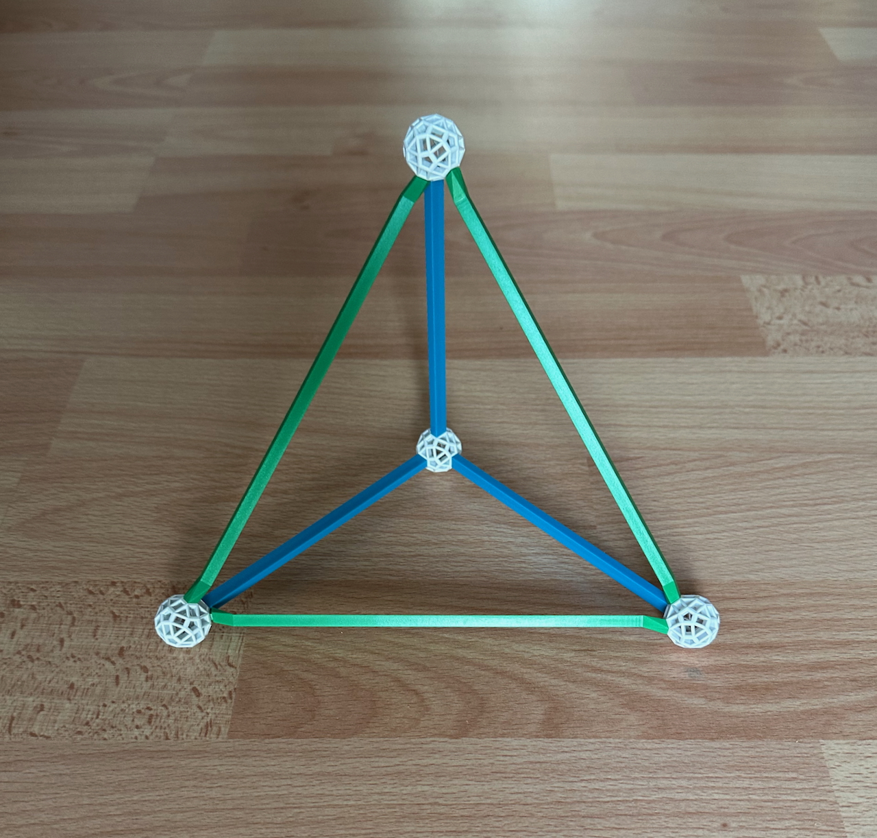
Fig. 9.14: Model of the fundamental region of the demitesseractic symmetry. This model is
only approximate, since the actual Tetrahedron is a spherical tetrahedron, so the angles
at the outer vertices are slightly distorted.
Reflecting either of the three outer vertices in the Wythoff construction, we obtain the
vertices of the 16-cell, with half of the length of their edges coinciding with one of the
edges of the fundamental region, as for the regular polyhedra and polychora above -- in
this case one of the blue struts. The edges of the three 16-cells generated by this
symmetry intersect in the connector in the middle. This is the phenomenon of triality we have met when discussing
the regular polychoron compounds, see
especially Fig. 7.2b on the right. Thus, we see that the phenomenon of triality stems
directly from the 3-fold symmetry of the CD graph for the tesseractic symmetry.
Reflecting the vertex at the centre (using the large Triangular mirror) we obtain the
rectification of all three, the 24-cell. As in the case of the polyhedral rectifications
discussed above, its edge is inside the fundamental region, linking the vertex at the
center with its reflection closer to us. Thus, as in those rectifications, each edge is
shared by two neighbouring Goursat tetrahedra. Since the 24-cell has 96 edges, the
3-sphere is covered by 192 of these tetrahedra.
Note than when we choose one of the outer vertices to generate the 16-cell, the symmetry
is broken into a bilateral symmetry, with the plane of bilateral symmetry passing through
the chosen vertex. Dividing this Goursat tetrahedron in half along that plane we obtain
the Goursat tetrahedron for the Hexadecachoric symmetry of the 16-cell, thus 384 of the
latter are needed to cover the 3-sphere. When we choose the central vertex to be reflected
and generate the 24-cell, the whole figure has 3-fold symmetry. Dividing this tetrahedron
along the three planes of bilateral symmetry of the 3-fold symmetry (as in Fig. 9.2b), we
obtain six different regions, the Goursat tetrahedra for the Icositetrachoric symmetry of
the 24-cell. Thus 6 × 192 = 1152 of those tetrahedra are needed to cover the
3-sphere.
Paulo's polytope site / Next: Beyond the fourth dimension.