Beyond the fourth dimension

Coxeter, like Forsyte's character "Old Jolyon", "ached a bit from sheer love of it all, feeling perhaps, deep down, that he had not very much longer to enjoy it. The thought that some day - perhaps not ten years hence, perhaps not five - all this world would be taken away from him, before he had exhausted his powers of loving it, seemed to him in the nature of an injustice, brooding over his horizon. If anything came after this life, it wouldn't be what he wanted."
Commentary on the last years of Coxeter's life in "King of Infinite Space: Donald Coxeter, the Man Who Saved Geometry", by Siobhan Roberts.

What happens at dimensions higher than 4?

Regular polytopes

Before moving on, we need new terms when discussion polytopes in many dimensions. The general equivalent of a face in a polyhedron and a cell in a polychoron is a facet. This is the highest-dimensional element of the surface of a n-dimensional polytope (henceforth, a n-polytope), thus having n−1 dimensions. This is also the case for the vertex figures. The ridges are n−2-D elements of the n-polytope's surface. This is also the case for the edge figures. In a regular polytope, all surface elements of a particular dimension are not only identical, but the polytope also looks identical as seen from each instance of those elements. This implies that each of the n types of element corresponds to a particular overall n−1-D symmetry of the polytope.

In Euclidean spaces with more than 4 dimensions, the only regular polytopes are the aforementioned simplices, hypercubes and their duals, the cross polytopes, or ``orthoplexes", making therefore a total of 3 regular polytopes for each Euclidean n-dimensional (henceforth n-D) space. These polytope families are infinite, with members in all n-spaces. There are no analogues of Icosahedra/Dodecahedra or 600-cell/120-cell, there are no regular star polytopes either, and nothing like the 24-cell, which exists only in 4-D Euclidean space. In this way, one comes to appreciate the fact the latter are exceptional objects.

We now enumerate the basic characteristics of these families that will be important for understanding what follows, with 3-D examples in parenthesis:

Regarding the simplices, they always have the smaller number of elements possible for a polytope in their n-space. The n-simplex (e.g., a Tetrahedron, ...) is built from a n−1-simplex A (Triangle A) with side ℓ by adding a single point outside A's n−1-D hyperplane, at distance ℓ from all vertices of A (... a pyramid apex, where Triangle A is the base), and linking that point to all the others with n other n−1-simplices (... n = 3 additional Triangular faces). Thus, the n-simplex has n+1 vertices, n+1 facets, and both the facets and vertex figures are n−1-simplices. They are therefore self-dual. They have no central symmetry.
The n-orthoplex (e.g., an Octahedron) is built from a n−1-orthoplex A (Square A) with side ℓ by adding two points, P1 and P2, in a line perpendicular to A's hyperplane at distance ℓ from A's vertices, one of them above and another one below A's hyperplane. Then those points are linked to A's vertices using n additional n−1-simplices for both P1 and P2, thus doubling the number of facets of A (... 2 × 4 = 8 Triangular sides). Importantly, P1 and P2 are not directly linked to each other. In this process A becomes an equatorial polytope. This implies that orthoplexes have 2n vertices and 2ⁿ facets.
The n-dimensional hypercube, or n-cube (e.g., a Cube) can be built from a n−1-cube A (Square A) with side ℓ by adding an identical n−1-cube, B, at distance ℓ from A along a perpendicular direction (... a second Square); this doubles the number of vertices. Then, A and B are connected with n−1-cubes, as many as the number of facets of A and B (... four additional Squares), in hyperplanes perpendicular to those of A and B. Thus, the number of facets grows by two with each dimension, their number is 2n; the number of vertices is 2ⁿ.

The n-orthoplex is the dual of the n-cube. They therefore share the same symmetry, which includes central symmetry. The n−1-simplex facets of the former correspond to the n−1-simplex vertex figures of the latter. The n−1-hypercubic facets of the latter correspond to the n−1-orthoplex vertex figures of the former. Since only the latter elements have central symmetry, only the orthoplexes have equatorial polytopes and only the Hypercubes have the dual equatorial facet rings. The n-orthoplex has an equatorial n−1-orthoplex between any two opposite vertices, their number is therefore 2 n / 2 = n.

***
We now present some Zomable projections of higher dimensional regular polytopes into three dimensions. Apart from their intrinsic interest, studying these projections will improve our understanding of projections of polytopes in general, and will add new understanding of the models of the 4-dimensional polychora as well. In all these models, the white connectors indicate real vertices, the other colours denote edge intersections that happen because of the projection, not in the polytopes themselves, which are all convex.

We start with the simplexes. When projecting a n-simplex into 2-D space, we can always arrange the direction of the projection in a way that the vertices are all equidistant from the centre. The reason is that, as we've seen above, when we build the n+1-simplex, we add a new vertex that lies on a line perpendicular to the n-simplex and is equidistant from all its vertices. Thus, if we project the n-simplex into 2-D space along that perpendicular line, then all its vertices must lie at the same distance from the centre. Furthermore, they and their connections to other vertices must look identical independently of the vertex, this implies a symmetric projection. Their distribution would be a regular Polygon with n+1 sides. To project the n+1-simplex, there are two easy options: one of them would be to project the new vertex to the centre (i.e., using the same projection vector as the previous projection), or project all vertices as the vertices of a n+1 Polygon.

For projections into three dimensions, the logic is the same, except that we can't find symmetries with an arbitrary number of vertices. For instance, for the 4-simplex, which has 5 vertices, there is no symmetric distribution of all vertices around the centre: what was done in Fig. 5.3 was to use a symmetric distribution of vertices of the 3-simplex (the Tetrahedron) and project the new vertex to the centre. The other Zomable projections of the 5-cell (Fig. 7.8) have a lower symmetry.

However, the 5-simplex has 6 vertices and 6 facets; this means that we can choose the direction of the projection in such a way that the vertices are equidistant from the centre as the vertices of an Octahedron.

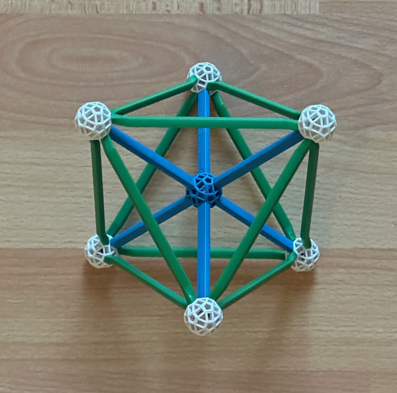
Fig. 10.1: An Octahedral projection of the 5-simplex.

In all simplices, the edges connect all vertex pairs, and in this model vertices and edges are shown without superposition. Thus, the model in Fig. 10.1, which is an accurate model of the Octahedral projection of the 5-simplex to three dimensions, resembles the vertex-first projection of the 16-cell in Fig. 5.4, with the difference that there are no vertices at the centre.

The 6-simplex has 7 vertices and 7 facets. For this, we can make a projection that uses the same projection vector as the projection in Fig. 10.1, this will place the additional vertex at the centre of the model. That projection would then be identical to that of the vertex-first projection of the 16-cell in Fig. 5.4. There would be 6 new blue edges connecting that vertex to all others, which will be superposed on the three blue edges of the previous model. This would be an analogue of the projection of the 5-cell in Fig. 5.3. The same strategy can be applied for the remaining projections of n-simplexes without central vertices to make projections of n+1-simplexes.

By the same logic used in the 5-simplex, it is easy to make a symmetric projection for the 7-simplex, which has 8 vertices and 8 facets. We can choose the direction of the projection in such a way that the vertices are distributed as the vertices of a Cube.

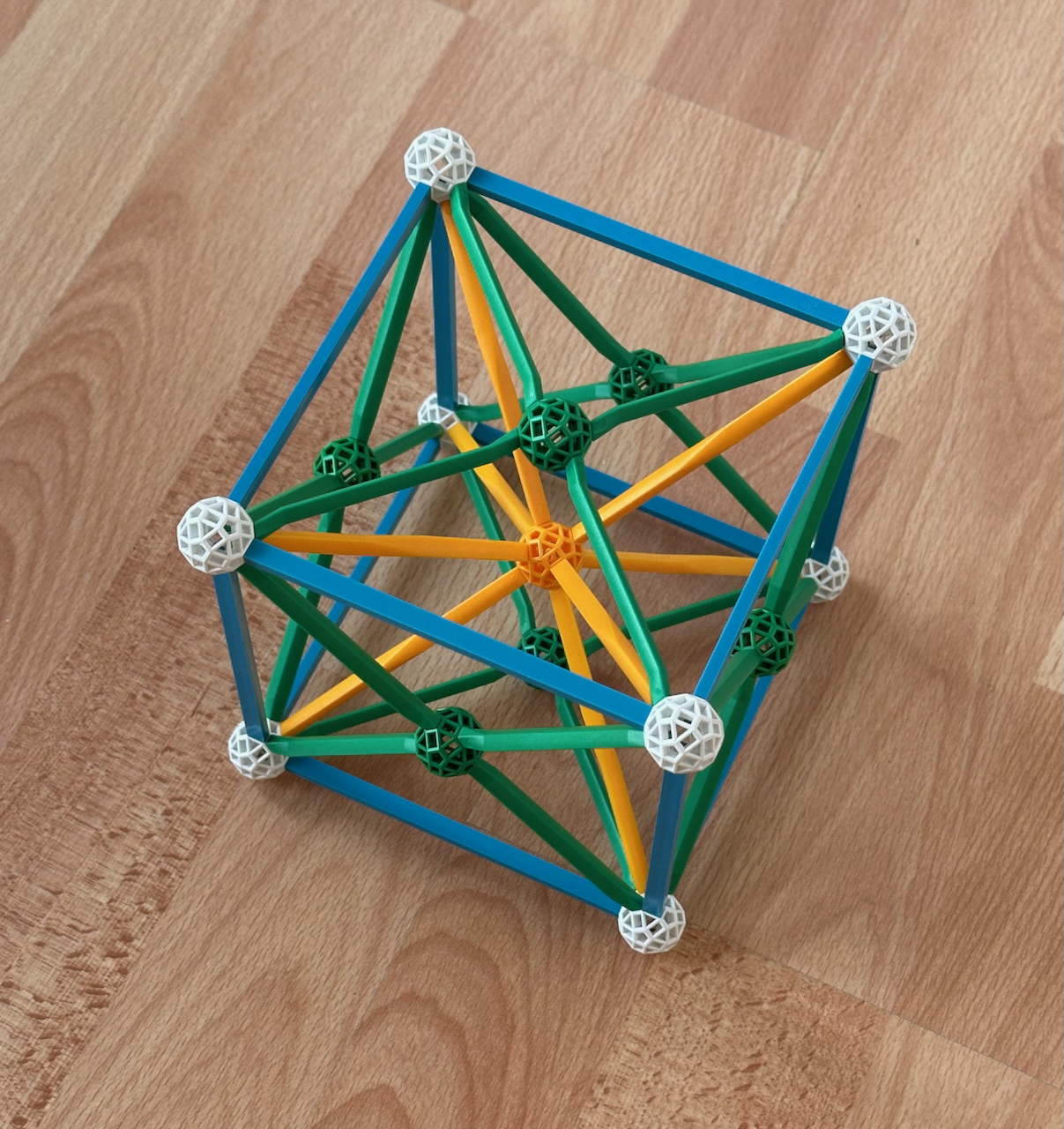
Fig. 10.2: An Octahedral projection of the 7-simplex.

Again, the edges connect all vertex pairs. Thus, the model in Fig. 10.2, which is an accurate model of the Octahedral projection of the 7-simplex to three dimensions, resembles the model of the Cube and its faceting in Fig. 4.5b, with the difference that there are four yellow edges connecting pairs of opposite vertices.

The 11-simplex has 12 vertices and 12 facets. We can choose the direction of the projection in such a way that the vertices are distributed as the vertices of an Icosahedron.

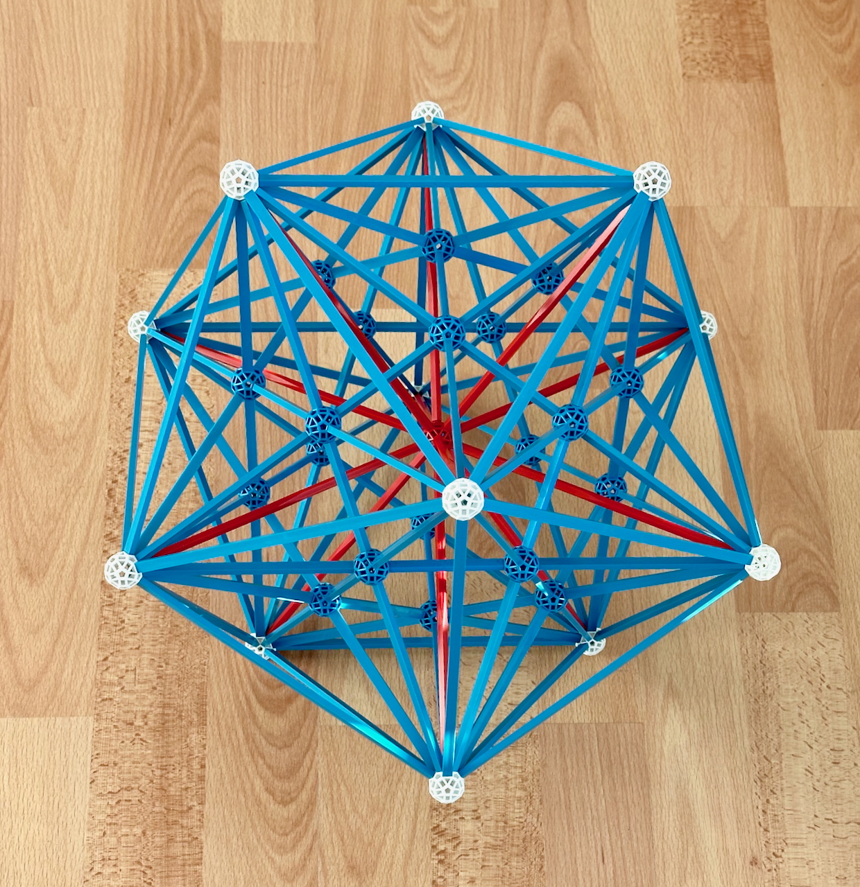
Fig. 10.3: An Icosahedral projection of the 11-simplex. This model required 30 B3 struts and 12 R3 struts, but this can avoided by building the model on a smaller scale, as in Fig. 4.6c.

Again, the edges connect all vertex pairs. Thus, the model in Fig. 10.3, which is an accurate model of the Icosahedral projection of the 11-simplex to three dimensions, resembles the model of the Icosahedron and its facetings in Fig. 4.6c, with the difference that there are 6 red edges connecting pairs of opposite vertices.

One could in principle make additional Icosahedral projections of the 19-simplex, for which the 20 vertices would have the distribution of the vertices of the Dodecahedron and have 10 yellow edges connecting pairs of opposite vertices, or of the 29-simplex, for which the 30 vertices would have the distribution of the vertices of the Icosidodecahedron and would have 15 blue edges connecting pairs of opposite edges. Their models would resemble, respectively, the models of the Dodecahedron and its facetings (Fig. 4.8) plus yellow radials and of the Icosidodecahedron and its facetings (Fig. 4.12) plus blue radials. However, as we'll see below, these projections are not Zomable.

***
The same idea used to make symmetric projections of the simplexes can also be used to make symmetric orthographic projections of the orthoplexes. The reason is identical to that used in the simplexes: when we build a n+1 orthoplex from a n-orthoplex, we add, in a line perpendicular to the n-orthoplex, two new vertices that are equidistant from all vertices of the n-orthoplex. This means that, when projecting the n-orthoplex along that perpendicular line, all vertices must lie at the same distance from the centre. The cell-centred projection of the 16-cell on the lower left of Fig. 5.4 is of this kind. Its 8 vertices are arranged symmetrically, which implies they are arranged as the vertices of a Cube. As remarked then, this projection is especially good for showing all the vertices separately. This makes it possible to see that the edges - all shown without superpositions as well - connect all vertex pairs except opposing vertices, as in all orthoplexes (this can more easily be seen in the Octahedron).

Projecting the n+1 orthoplex along the same projection vector would add the two new vertices to the centre of the projection. The vertex-first projection of the 16-cell in Fig. 5.4, where two new vertices were added at the centre of an Octahedron, is of this kind. Using the same logic, we can represent the 5-orthoplex by using the same projection vector as in the cell-first projection of the 4-orthoplex (the 16-cell) and adding two new vertices, which would appear superposed at the centre (see Fig. 10.4). These don't connect to each other, but connect to all others via Y struts. The same strategy can be applied for the remaining projections of n-orthoplexes without central vertices to make projections of n+1-orthoplexes.

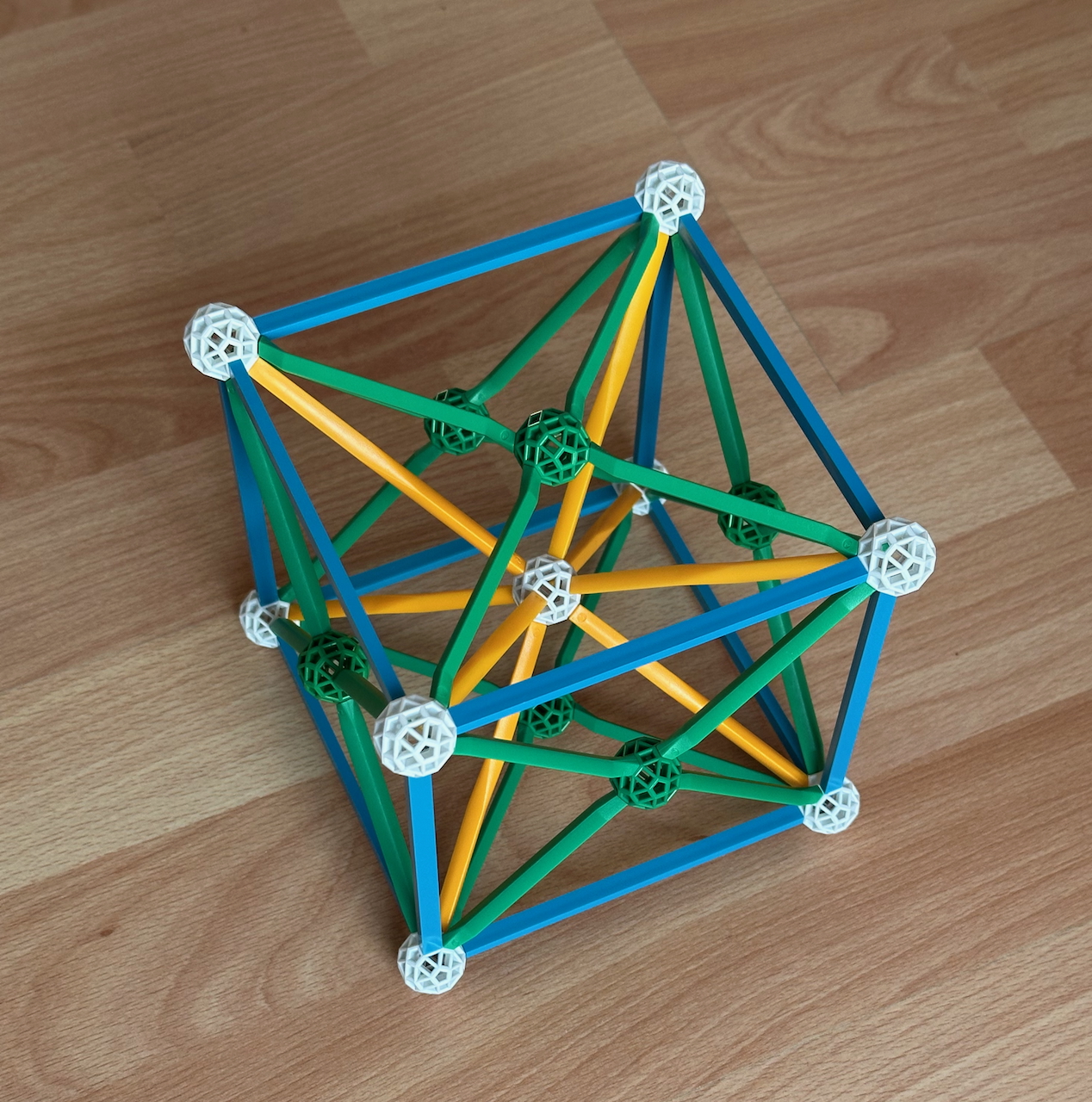
Fig. 10.4: An Octahedral projection of the 5-orthoplex.

Fig. 10.5 shows the 6-D analogue of the cell-first projection of the 16-cell in Fig. 5.4, the Icosahedral projection of the 6-orthoplex. In this projection, the 2 × 6 = 12 vertices are arranged symmetrically, i.e., as the vertices of the Icosahedron. Again, all vertices are shown without superpositions. This allows us to see that, again, the edges, which are also shown without superpositions, connect all vertex pairs except opposing vertices. This makes the model different from the model of the 11-simplex in Fig. 10.3, where the red radials were fulfilling that role, but identical to the model of the Icosahedron and its facetings in Fig. 4.6c.

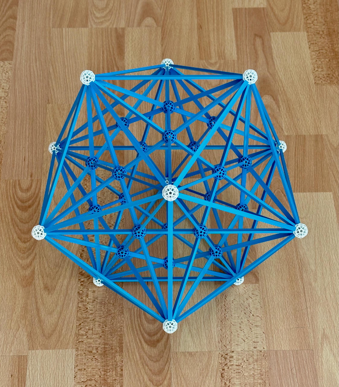
Fig. 10.5: The Icosahedral projection of the 6-orthoplex. This projection used 30 B3 struts.

This polytope has 60 edges (the 30 of the outer Icosahedron plus the 30 of the inner Stellated dodecahedron), 160 Triangular faces, 240 Tetrahedral cells, 192 5-cell ridges and 2⁶ = 64 5-simplex facets.

In the Icosahedral projection of the 10-orthoplex, the 20 vertices will be distributed as the vertices of a Dodecahedron, and the edges will connect all vertex pairs, except opposing vertices. Thus, the projection will look very similar to the model of the Dodecahedron and its facetings in Fig. 4.8, with B and G struts, only with the difference that instead of a Compound of five tetrahedra, a Compound of ten tetrahedra would be needed, so that all non-opposing vertices are connected. However, as remarked after Fig. 4.7b, this compound is not Zomable.

The Icosahedral projection of the 15-orthoplex would have its 30 vertices distributed as the vertices of the Icosidodecahedron. The edges connect all vertex pairs, except opposing vertices; the resulting projection would look somewhat like the model of the Icosidodecahedron and its facetings in Fig. 4.12, except that it would require three additional edge directions that are not Zomable.

***
For hypercubes, the reasoning used above to make the projections no longer applies: when building a n+1 cube from a n-cube, not all vertices of the n-cube are equidistant from the new vertices of the n+1 cube. For that reason, the strategy used to make the projections must be different. The strategy to be adopted is based on the fact that for a n-cube, there are only n edge directions. Since an orthographic projection is an affine projection (which preserves parallelism), a projection of a n-cube will also have only n distinct edge directions.

This implies that several projections of higher-dimensional hypercubes are not only Zomable, but also Zomable in a single colour, with the models having a high degree of symmetry. The reason for this can be understood from the study of the models of the Cube and Tesseract.

The three axes of the Cube can be represented in 3 dimensions without distortion, in three orthogonal directions, all with blue struts. If we want to project it in two dimensions, we can choose to project all edge directions equally, in which case they must have a symmetrical Triangular arrangement (see Fig. 5.2, model B). All edges are represented with the same length, and all vertices connect to three edges, which represent the full set of edge directions.

Similarly, for the Tesseract, we cannot represent the four axes as orthogonal directions in 3-D space, but we can choose to represent them equally, which implies a symmetric arrangement - in this case the radial struts of a Tetrahedron, all of which are Y struts (see Fig. 4.3a). This is the vertex-first projection of the Tesseract in Fig. 5.4. All edges are represented with the same length, and all vertices connect to four edges, which have the full set of edge directions.

For the 6-cube, we can also make an orthographic projection to three dimensions and treat all 6 edges directions equally (implying also symmetrically) by making them parallel the six axes of symmetry of the Icosahedron, which are represented in the Zometool by the R struts. A model of this projection is shown in Fig. 10.6. This is the dual of the projection of the 6-orthoplex in Fig. 10.5. All vertices connect to 6 struts, which represent the full set of edge directions in the model.

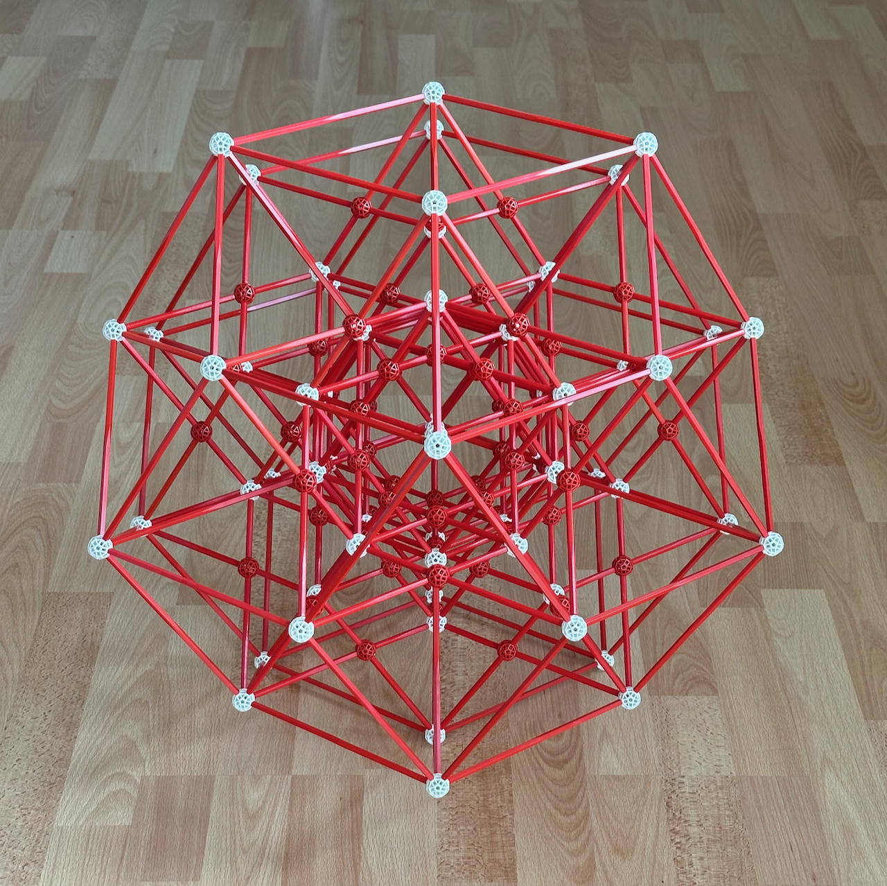
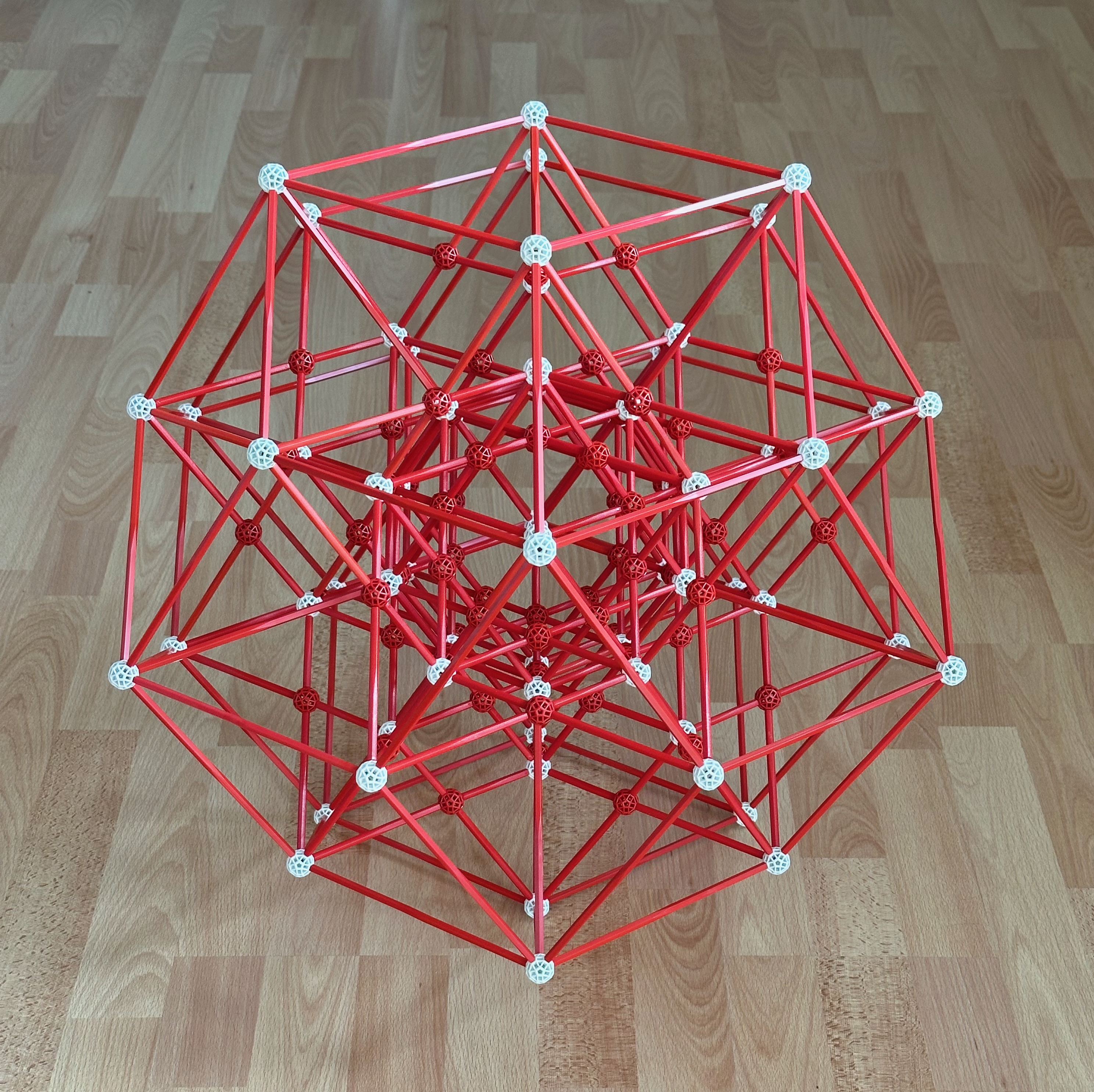
Fig. 10.6: An Icosahedral projection of the 6-cube, the dual of the 6-orthoplex. This is the dual of the Icosahedral projection of the 6-orthoplex in Fig. 10.5.

I made this model with the help of a vZome model made by Scott Vorthmann. This projection uses 72 R3 struts. To avoid this, the model can be built on a smaller scale using R00 struts.

All elements are the duals of the elements of the 6-orthoplex in Fig. 10.5. The 12 5-cubic facets correspond to the the vertices of the 6-orthoplex, like them their projections are all identical and are associated with the 6 axes of 5-fold symmetry of the model. The 60 Tesseractic ridges are perpendicular (in 6 dimensions) to the edges of the 6-orthoplex; the 160 Cubic cells correspond to the latter's 160 Triangular faces, the 240 Square faces, which are all projected in the same way (as Golden rhombuses), correspond to its 240 Tetrahedral cells, the 192 edges are perpendicular to its 192 5-cell ridges and 64 vertices correspond to its 64 5-simplex facets. The Golden rhombuses of this projection are analogous to Yellow rhombuses of the vertex-centred projection of the Tesseract.

Note also how much larger the projection is relative to the size of the edge, a phenomenon we had already see in Figs. 5.2 and 5.4. The reason is counter-intuitive: although the "side" of a unit n-cube is always 1, the distance to the center (√n/2) increases without bound with n. However, unlike those projections, this is not a vertex-first projection. In this model, we start to see that projecting objects from dimensions higher than four into three dimensional space leads to a concentration of vertices and edges near the centre.

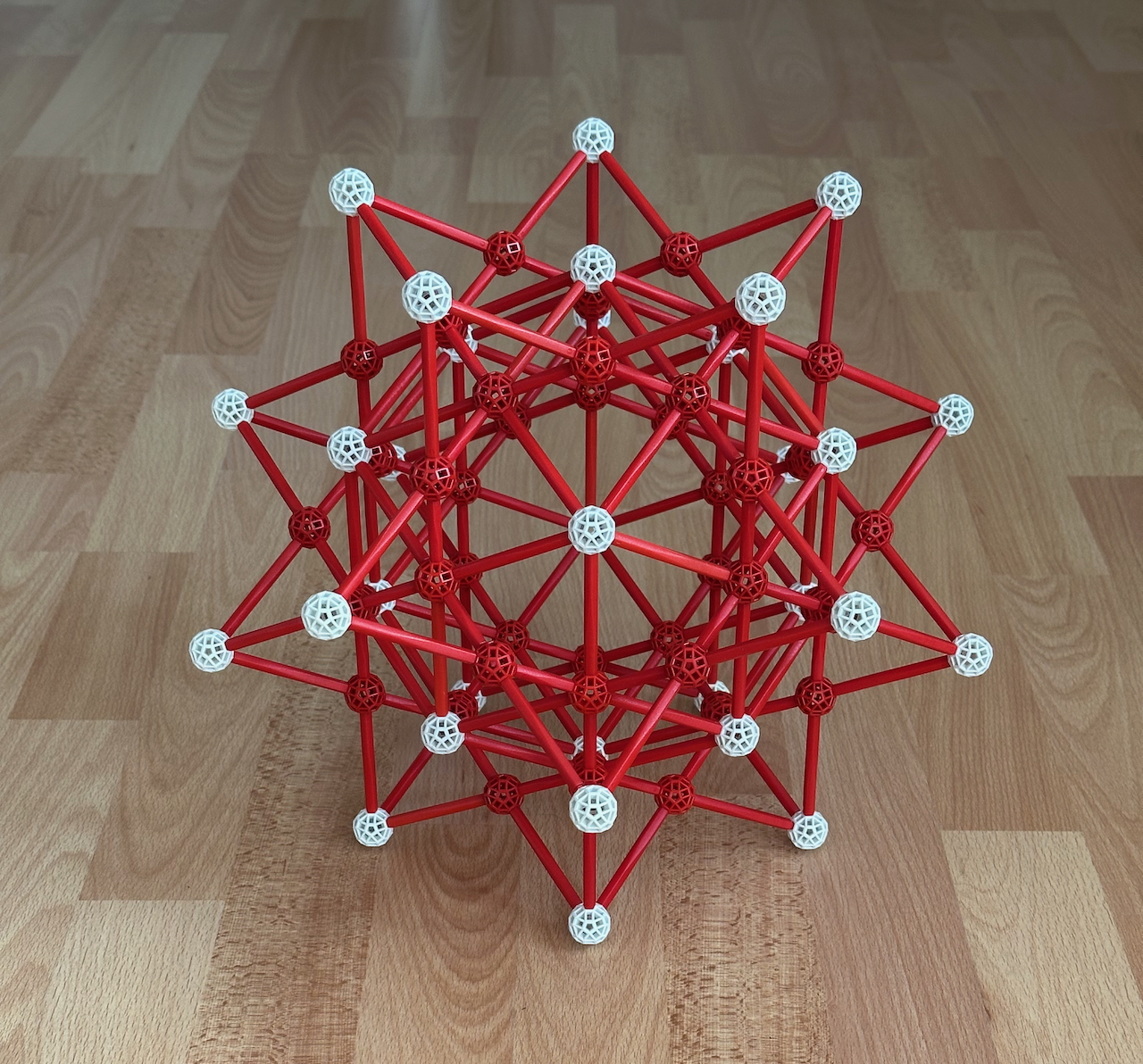
Fig. 10.6a: The Great rhombic triacontahedron.

To build the model in Fig. 10.6, we start by building a core with the vertices and edges of the Great Rhombic triacontahedron (Fig. 10.6a). Perhaps this is the reason why this pair of polytopes appears in the cover of Coxeter's ``Regular Polytopes".

Any orthographic projection of a hypercubic element into a plane will be circumscribed by a polygon with central symmetry, where, as in the original hypercube, each edge has an opposite edge that is parallel to it. Any orthographic projection of any n-cube will therefore be bound by a polyhedron with this type of faces: the aforementioned zonohedra. The characteristics of their faces imply that all faces are part of face rings, each containing a particular edge direction that does not exist outside that ring, each of these corresponds to one of the directions of the edges of the hypercube.

In the case of the projection in Fig. 10.6., the envelope is a zonohedron with Icosahedral symmetry that is constructible with R struts and has Golden rhombic faces, which are projections of Square faces. We have seen this object before, it is the Rhombic triacontahedron. This situation is analogous to the envelope of the vertex-first projection of the Tesseract in Fig. 5.4, a Zonohedron with Octahedral symmetry and Yellow rhombic faces (also the projections of Square faces) that can be represented with Y struts, the Rhombic dodecahedron. Just as the vertex-first projection of the Tesseract showed the parallelism between the yellow radials of the Cube (Fig. 4.3a) and yellow edges of the Rhombic dodecahedron, the model in Fig. 10.6 shows the parallelism between the red radial edge directions of the Icosahedron (Fig. 4.2) and the red edges of the Rhombic triacontahedron.

Fig. 10.6b: My Big Ball of Whacks (6-color edition), with each colour showing five of the ten faces in each equatorial ring. Each colour is associated with a single edge direction, which is perpendicular to that ring.

There is a magnetic toy puzzle that can be arranged as a Rhombic triacontahedron, the Big ball of whacks. The pieces come in six colours. At first I was wondering why six: with five colours, it would have been easier to create symmetrical patterns. However, I could find a pattern where the five Golden rhombuses of each of the six colours covers half the faces of a particular equatorial ring of 10 faces (each of the 30 faces belongs to two rings). For each of these colours/rings there is a single edge direction that is common to all the faces in the same ring, and perpendicular to the ring itself (see Fig. 10.6b); this edge direction is absent outside this ring. This is a very nice general illustration of the concept of a Zonohedron, and in this case of the 6 edge directions of the projection of the 6-cube in Fig. 10.6.

The same logic can be applied to projections of some higher-cubes. An an example, if during an orthographic projection to 3-D space we treat all 10 edge directions of the 10-cube equally and therefore symmetrically, we must make them parallel to the 10 axes of 3-fold symmetry of the Dodecahedron. Since these are represented in the Zometool by Y struts (see Fig. 4.3c), this results in a yellow projection of the 10-cube with full icosahedral symmetry (see Scott Vorthmann's vZome model here). This projection is so complex that it is impractical to make a physical model of it with the Zometool. However, its envelope is simple (see Fig. 10.7); it is the largest Zomable yellow zonohedron, the rhombic enneacontahedron. This has 10 edge directions, and thus 10 face rings, 5 yellow rhombuses around each of the 12 vertices in the 6 axes of 5-fold symmetry, and 30 long yellow rhombuses centred on the axes of 2-fold symmetry.

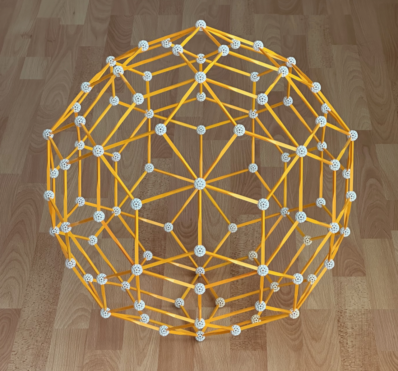
Fig. 10.7: The Rhombic enneacontahedron. This zonohedron is the envelope of the Icosahedral projection of the 10-cube.

If, in an orthographic projection of the 15-cube to 3 dimensions we treat all its 15 edge directions equally, we must make them parallel to the 15 axes of 2-fold Icosahedral symmetry, resulting in a blue projection of the 15-cube with full icosahedral symmetry. Its envelope is the largest blue zonohedron that can be represented with the Zometool, the Truncated icosidodecahedron.

This logic continues for higher dimensions: we can still make symmetrical models, but now we can no longer treat all edge directions equally. Any Zomable zonohedron corresponds to a Zomable projection of a Hypercube. Given that the Zometool connector has 31 axes of symmetry (6 red, 10 yellow and 15 blue), it can theoretically represent an Icosahedral projection of a 31-cube. While that projection itself is practically impossible to make, its zonohedral envelope is relatively simple.

Finally, we should also remark that a simple Cube (n = 3) also represents projections of all n-cubes with n > 3, where all other dimensions are reduced to points (an example of this is the cell-first projection of the Tesseract in Fig. 5.4). The same applies to all other models of n-cubes in this site.

Semi-regular polytopes

As we remarked when discussing the partially regular polychora, associated with the orthoplexes are the non-convex demicrosses. The facets of the n-demicross are half of the 2ⁿ n−1-simplex facets of the n-orthoplex plus its n equatorial n−1-orthoplexes; the vertex figure is the n−1-demicross; all other elements are as in the n-orthoplexes. This works because, as mentioned above, the vertex figures of the n−1-simplices and orthoplexes are, respectively, n−2-simplices and orthoplexes. The identical vertex and edge arrangements imply that all Zometool projections of n-orthoplexes in this site also depict n-demicrosses. The demicrosses have a special characteristic of being non-orientable.

There is a related infinite family of convex uniform polytopes, the aforementioned demicubes. The demicrosses are obtained by removing alternate facets of orthoplexes; the demicubes are convex polytopes obtained removing alternate vertices of the duals of the orthoplexes, the hypercubes. This implies that the demicrosses share the symmetries of the demicubes. The operation of removing half of the vertices of a n-cube to form a n-demicube forms an equal number (2ⁿ⁻¹) of n−1-simplices under the removed vertices, the reason is that they are the vertex figures of the n-cube; this can be visualised easily in the case of the formation of a Tetrahedron from a Cube. The subtraction of alternated vertices from the 2n n−1-cubic facets transforms them into 2n n−1-demicubic facets. The number of n−1 simplices and their arrangement is the same in a n-demicube and n-demicross.

A consequence of the formation of the demicubes from hypercubes is that we can do the same for the hypercubes from a hypercubic honeycomb to form a demicubic honeycomb, in which the facets are demicubes and (centered on the deleted vertices) orthoplexes. Therefore, in general, these honeycombs are not regular.

The demi-hypercubic family is thus far hidden because, as we've seen here, all uniform polyhedra and polychora that have their symmetries already exist as members of other families, two of them being regular: the demi-Cube is the Tetrahedron (where the demi-cubic facets are 2-sided "polygons", the edges of the Tetrahedron, in this case we only see the 2-simplex faces) and the demi-Tesseract is the 16-cell - this is regular because both the 3-demicube and the 3-simplex facets are identical (Tetrahedra). The same happens to the demicubic honeycombs: In 3 dimensions, this is the Tetrahedral- Octahedral honeycomb; in 4 dimensions it coincides with the 16-cell honeycomb: this is regular because the 16-cell is both a demicube and an orthoplex.

It is only in 5 dimensions that we find new polytopes that have the demi-hypercubic symmetry as their highest symmetry. Of special interest is the 5-demicube, which has 10 16-cells and 16 5-cells as facets; this makes it semi-regular. But, despite the fact that this family is infinite, the list of demicubes that are either regular or semi-regular ends here! Interestingly, all n-demicrosses (which have the same symmetry) are not only semi-regular, with n−1 simplices and orthoplexes as facets, but also (as defined in this site) partially regular: a semiregular faceting of a regular polytope.

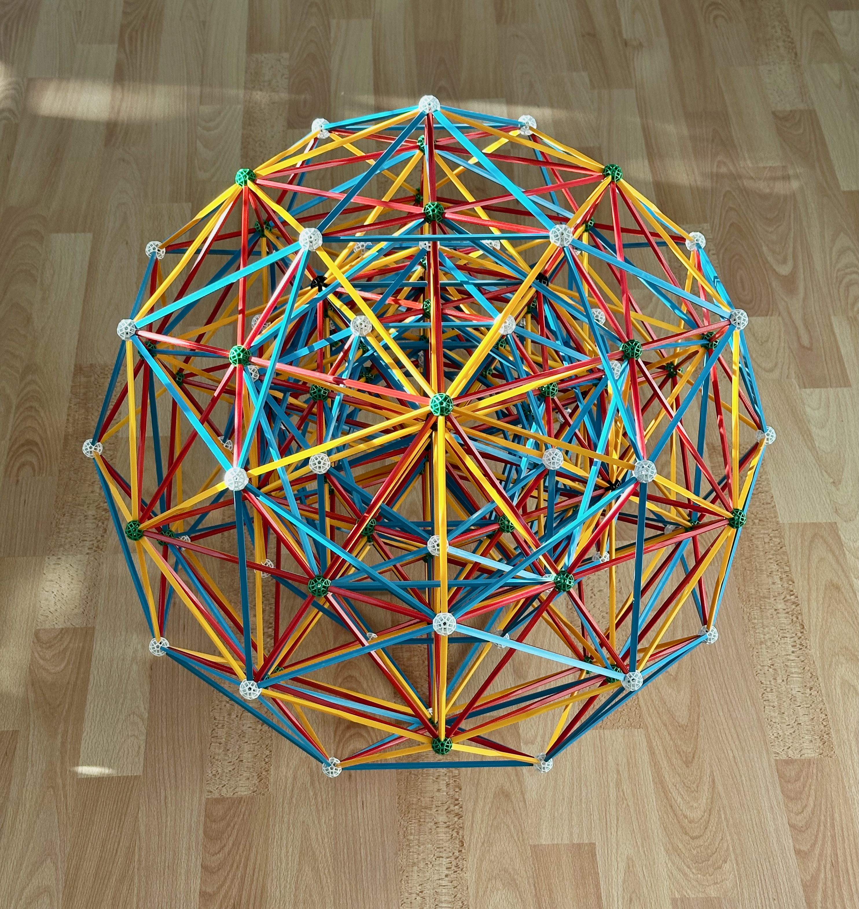
The next member of the family is the uniform 6-demicube. Like the 6-orthoplex and 6-cube, this has a beautiful Icosahedral projection (see Fig. 10.8).

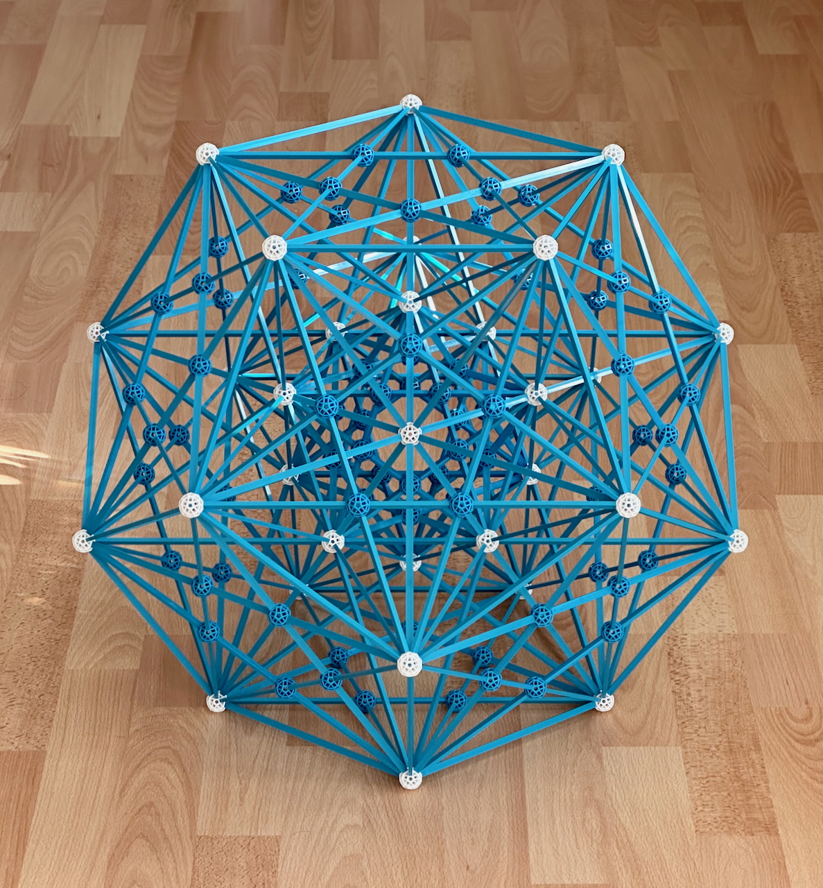
Fig. 10.8: One of the two Icosahedral projections of the 6-demicube.

The projection cannot be represented on a smaller scale, because it uses B0 struts. The model requires the use of 90 B3 struts.

In the formation of a n-demicube from a n-cube, all m-cubic (with 1 < m < n) elements become m-demicubes. Thus, in the case of of the transformation of the 6-cube into a 6-demicube, the 12 5-cube facets of the former are replaced by 12 5-demicubes, its 60 Tesseract ridges are replaced by 60 16-cells, its Cubic cells are replaced by Tetrahedral cells and the 240 Square faces become 2-demicubes, which as mentioned in the case of the Tetrahedron are 2-sided polygons - the full set of 240 edges of the 6-demicube. These are one set of diagonals of the Square faces of the 6-cube. Under the 32 vertices of the 6-cube that disappeared, 32 new 5-simplex facets appeared, which are the vertex figures of the 6-cube. These have 32 × 6 = 192 5-cell ridges, as many as the edges of the 6-cube; the 5-cell is the edge figure of the 6-cube. The vertex figure is the Rectified 5-simplex.

We now discuss edge models of demicubes. In Fig. 4.5b, on the right, we see how the transformation of a Cube into a demicube (Tetrahedron) depends on the choice of vertices we "delete", i.e., of how we bisect the Squares. In Fig. 5.4, both projections of the 16-cell result from bisecting the vertex-first projection of the Tesseract. They represent the two choices of diagonals of Square faces of the Tesseract, which in the projection appear as Yellow rhombuses: if we choose the longer diagonals (G struts) of the outer rhombuses, we obtain the vertex-centred projection of the 16-cell (which include the shorter radials), which has an Octahedral envelope; if we choose the shorter diagonals (B struts) we obtain the cell-first projection of the 16-cell, which has a Cubic envelope.

To make Icosahedral projections of the 6-demicube with the Zometool, we start from the Icosahedral projection of the 6-cube in Fig. 10.6 and bisect all Square faces, all of which are projected in that model as Golden rhombuses. As seen in Fig. 4.9 both diagonals of a Golden rhombus can represented by B struts; for that reason, the two Icosahedral projections of 6-demicubes will be entirely represented by B struts. In the projection in Fig. 10.8 we choose the smaller diagonals of the outer Golden rhombic faces; this results in a projection with a Dodecahedral envelope. The second projection, where we choose the longer diagonals of the outer Golden rhombic faces, has an Icosahedral envelope. Interestingly, both projections would look exactly the same when seen from a 5-fold symmetry axis!

The projection in Fig. 10.8 is notable for having the edges of the model of the stellations of the Dodecahedron (Fig. 4.6b) and the model with its facetings (Fig. 4.8), with the exception of the Compound of five tetrahedra.

***
To proceed, we will need to discuss the properties of some of the higher-dimensional symmetry groups. For the linear CD graphs of the Simplexes, Hypercubes and Orthoplexes, ringing a single node at either end generates a regular polytope. As we've seen for the 3-branch graph of the 4-D demicubic symmetry, ringing any single node creates a regular polychoron, either a 16-cell or a 24-cell. However, for other 3-branch graphs this is generally not the case, as discussed below, even though their Wythoff constructions are identical to those of the regular polytopes.

For such "Wythoff-regular" polytopes, Coxeter introduced a handy, compact notation. This consists of three numbers, which are the lengths of the branches of the CD graph, none of which includes the central node. The sum of their lengths must therefore be the dimension of the polytope − 1 (which accounts for that central node). The first number designates the length of the branch for which the end node is being ringed. The lengths of the other two branches are indicated in subscript. For polytope k_ij, the cells are k_(i−1)j and k_i(j−1) polytopes and the vertex figure is a (k−1)_ij polytope.

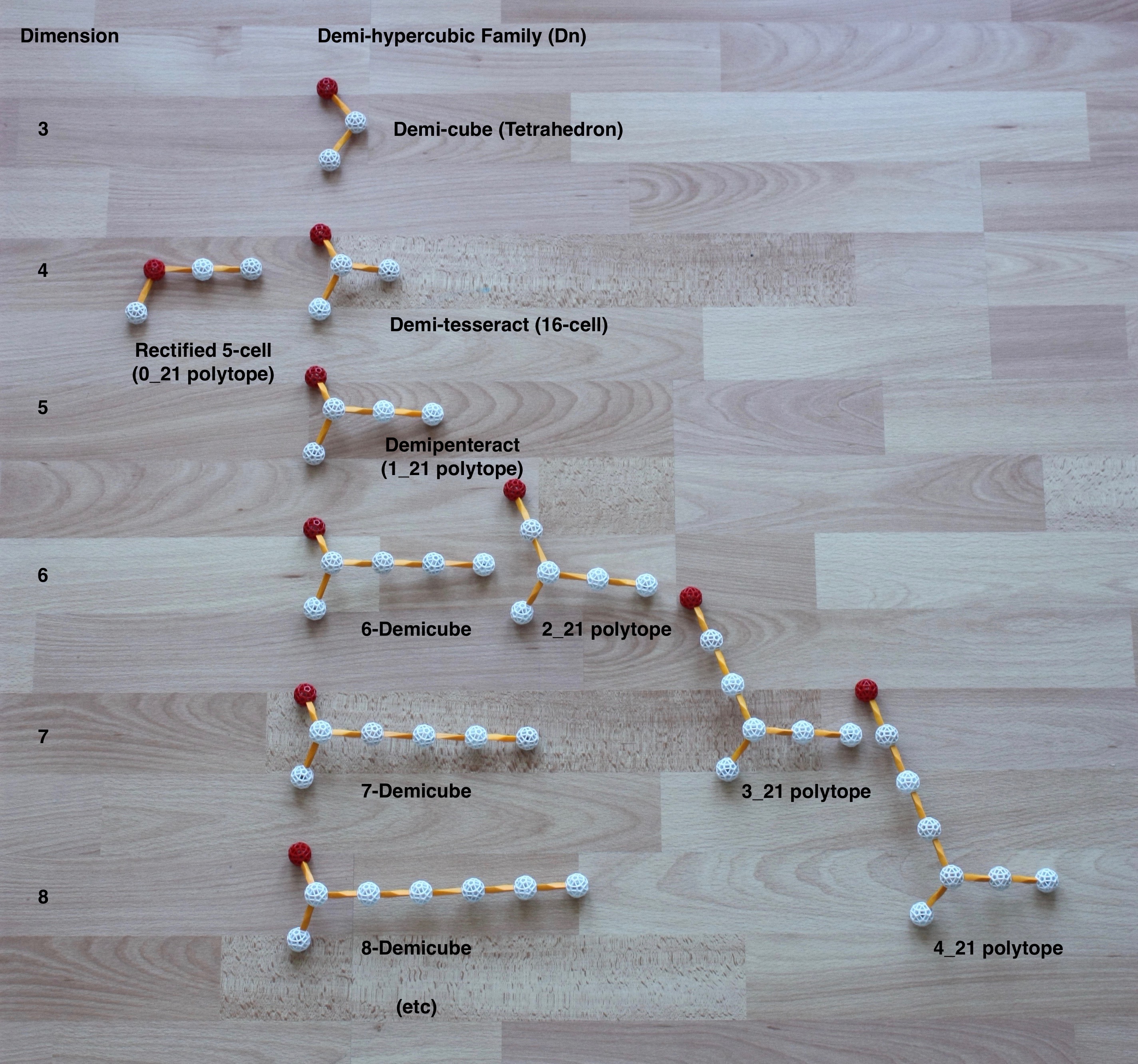
The CD graphs of the demicubic symmetries can be seen arranged in a column in Fig. 10.9. They always have two branches of length one and a branch of arbitrary length. The demicubes result from ringing the node at one of the branches of length one (in black) - they are therefore, in Coxeter's notation, 1_k1 polytopes. Their facets are either 1_(k−1)1 polytopes - the n−1-demicubes - or 1_k0 polytopes, which are linear chains ringed at one end, the simplexes.

Fig. 10.9: The CD graphs for the demicubes (vertical column), rectified 5-cell (left) and three higher-dimensional semi-regular polytopes (right). The nodes being ringed are indicated by the red balls.

However, something interesting happens when we ring the last node of the long branch. This produces a k₁₁ polytope that has only simplex (k₁₀) facets. Also, as we see by cutting one node from the k-branch, this polytope has (k−1)₁₁ polytopes as vertex figures. From their structure in 3 and 4 dimensions, we find they are orthoplexes. Thus, as for 3 and 4 dimensions, the demicubic symmetries can always generate the orthoplexes.

***
The semi-regularity of the 5-demicube marks it as a member of a family of semi-regular convex polytopes with the same behaviour of the demicrosses, the k₂₁ polytope family. Their CD graphs are also shown in Fig. 10.9. As in the case of the orthoplexes above, the fact that in this family the node being ringed is the variable integer (k) implies that the k₂₁ polytope is the vertex figure of the (k+1)₂₁ polytope. That it is semi-regular can be seen by subtracting nodes from the other two branches: this produces k₂₀ polytopes (simplexes) and k₁₁ polytopes, the orthoplexes.

Like the demicrosses, this family exists because, as mentioned above, n-simplices and n-orthoplexes have, respectively, n−1-simplices and orthoplexes as vertex figures. The 0₂₁ polytope must be, as discussed above, 4-dimensional: as the name indicates (see also graph in Fig. 10.9), it is the Rectified 5-cell, a semi-regular polychoron with simplices (Tetrahedra) and orthoplexes (Octahedra) as cells. This is the vertex figure of a 5-D object with 4-simplices (5-cells) and 4-orthoplexes (16-cells) as facets: the 1₂₁ polytope, the 5-demicube.

Something extraordinary happens next. The 2₂₁ semi-regular polytope has 72 5-simplex and 27 5-orthoplex facets. What is unusual is its symmetry, which is quite unlike any we've seen until now; it is one of 39 uniform polytopes with E₆ symmetry. In seven dimensions, the 3₂₁ semi-regular polytope has 576 6-simplex and 126 6-orthoplex facets. It is one of 127 uniform polytopes with E₇ symmetry. Finally, in eight dimensions, the 4₂₁ semi-regular polytope (see Figs. 10.10 and 10.11) has 17280 7-simplex and 2160 7-orthoplex facets. It is is one of 255 uniform polytopes with E₈ symmetry. All E₈ polytopes have 696,729,600 symmetries, i.e., this is the number of fundamental simplexes in the E₈ kaleidoscope!

That's it! Unlike in the case of the demicrosses, the family ends, because its next member has an angular defect around each vertex of zero, being therefore a tesselation of the 8-D space, the 5₂₁ honeycomb. The fact that it is infinite implies that it cannot serve as a vertex figure for any higher-D polytope. From this, we conclude that the E₆, E₇ and E₈ symmetries are also exceptional objects!

Merely by rearranging which branch is ringed in the CD graphs of the k₂₁ family in Fig. 10.9., we obtain the 2_k1 and 1_2k polytope families, which include the exact same symmetries, both of which start with the 5-cell.

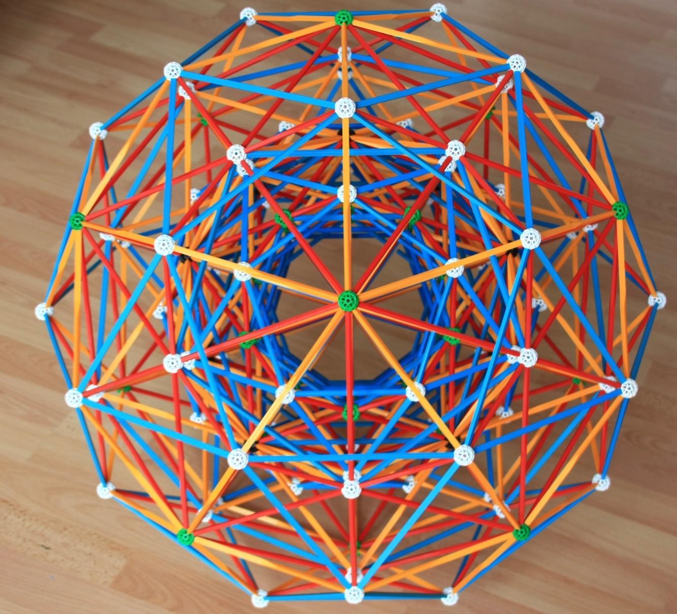
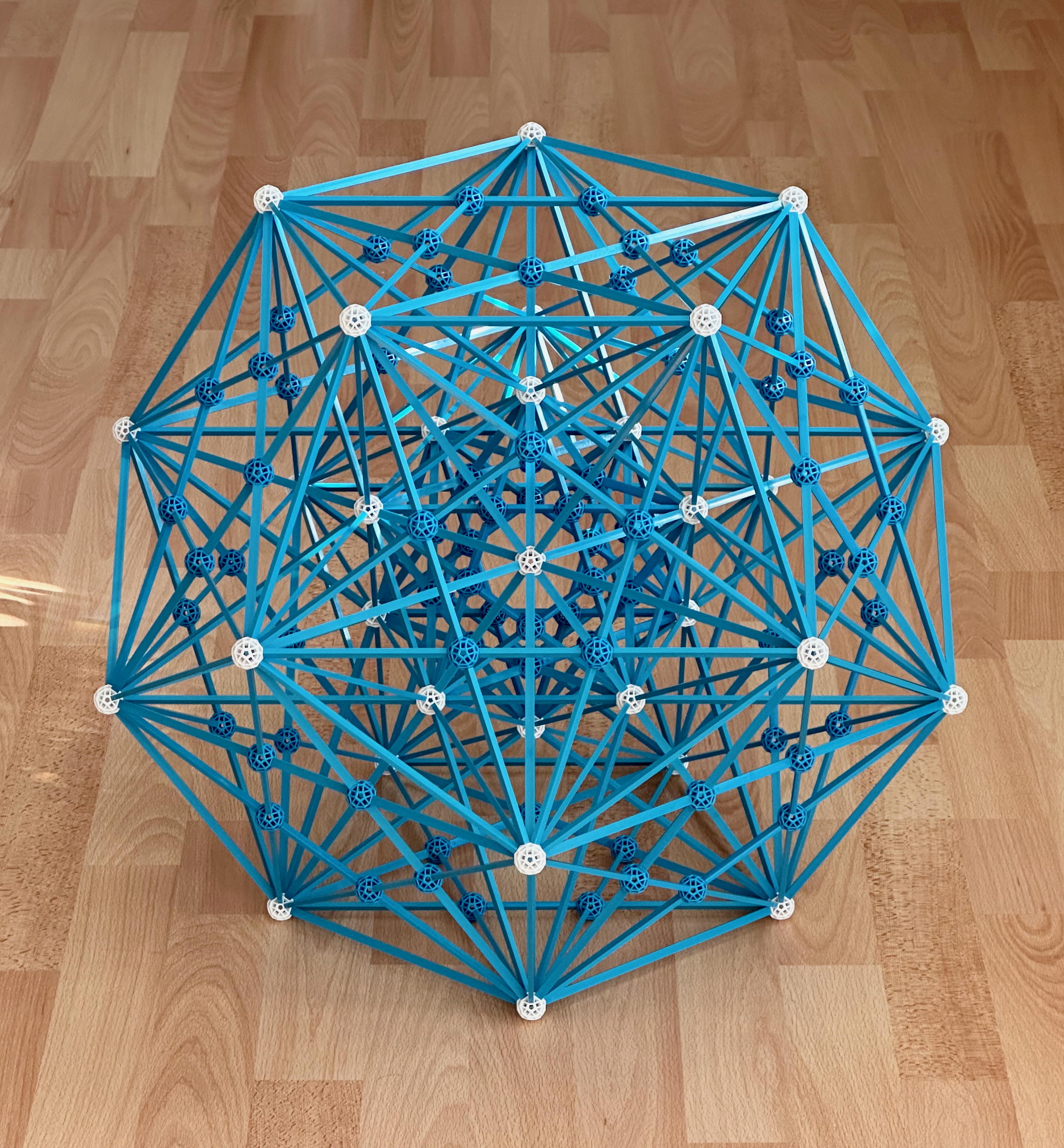
Fig. 10.10: A Zomable projection of the 4₂₁ polytope.
This model required 120 B3s, 60 R3s and 120 Y3s. Alternatively, the model can be made on a smaller scale.

Fig. 10.10 shows a Zomable projection of the 4₂₁ polytope that has Icosahedral symmetry. However, and importantly, it also represents a projection of the 4₂₁ polytope to 4-D space that has the Hexacosichoric symmetry of the 600-cell. This is highlighted by the fact that the 240 vertices project here as the 2 × 120 vertices of two concentric 600-cells, with one of them being larger than the other by a factor of φ. The reason for this is explained in detail here.

It is not possible to project all 6720 edges into a 3-D Zometool model: in this projection, they are all Zomable, but they just have too many intersections. Therefore, we must choose a subset of edges to represent. In this model, we use a beautiful fact, that projection of the 4₂₁ polytope into 4-D space also contains all 2 ×720 = 1440 the edges of those two concentric 600-cells.

This projection is analogous of the 3-D projections of the 6-cube, 6-demicube and 6-orthoplex to 3-D space that have Icosahedral symmetry, which is the 3-D version of the Hexacosichoric symmetry of the 600-cell.

For more on Zomable projections of k₂₁ polytopes, check this vZome page. For a physical Icosahedral projection of the 4₂₁ polytope with all edge directions represented, see Fig. 10.11.

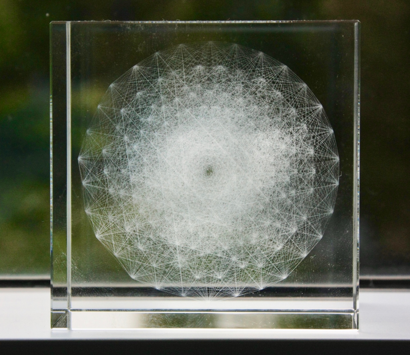
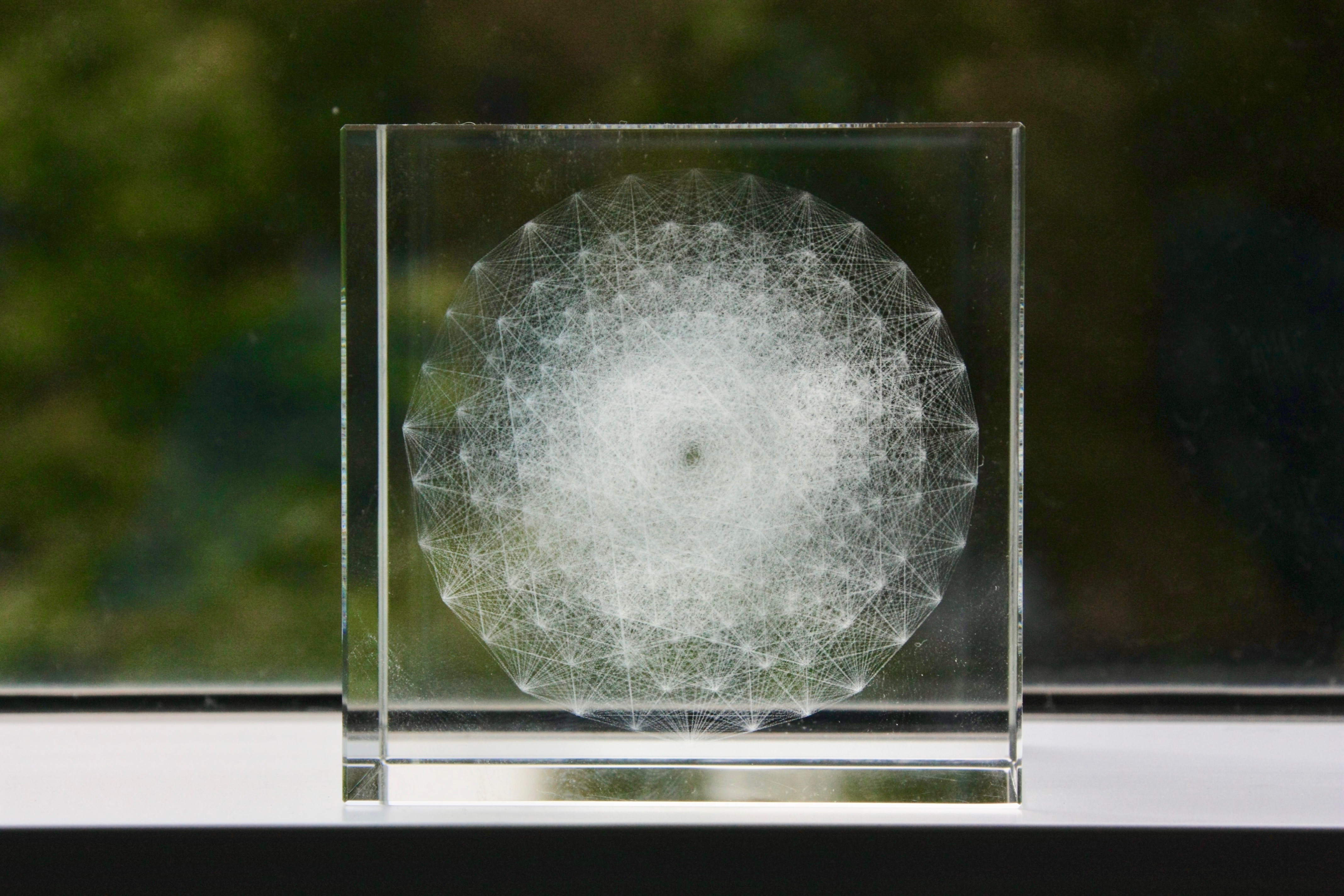
Fig. 10.11: An orthographic projection of the 4₂₁ polytope in 3-D space, now with all the edges represented. This model is laser-engraved in glass.
This was a present from one of my students, Jose Martinez.

The polytopes depicted in this page have a dense set of geometric relations. This is highlighted by the fact that, in addition to the previous polytope families, there are several others, which include some of the same objects. For instance, the 5-simplex alone belongs to 3 different multi-dimensional polytope families that start in 5 dimensions, where it is the case with k = 0:

The 1_3k polytope family. The 6-D member, the 1₃₁ polytope, is the aforementioned 6-demicube. The 7-D member, the 1₃₂ polytope, is one of the aforementioned 127 uniform polytopes built with E₇ symmetry; it facets are 1₂₂ polytopes and 6-demicubes. The family ends with the 1₃₃ honeycomb of 7-D space; this has only one type of facet, the 1₃₂ polytope.
By changing which branch is being ringed in the CD graphs of the last family, we obtain the 3_k1 polytope family, which has the same symmetries. The 6-D member, the 3₁₁ polytope, is the aforementioned 6-orthoplex. The 7-D member is the aforementioned 3₂₁ semi-regular polytope. The family ends with the 3₃₁ honeycomb of 7-D space, which has 3₂₁ and 7-simplex facets and the same symmetries as the 1₃₃ honeycomb.
The 2_2k polytope family. The 6-D member is the aforementioned 2₂₁ semi-regular polytope. The family ends with the the 2₂₂ honeycomb of the 6-D space, which has only one type of facet, the 2₂₁ polytope.

The last rearrangement of the first two families is the k₃₁ family (where, as it should be clear by now, each polytope is the vertex figure of the (k+1)₃₁ polytope). The 0₃₁ polytope is the rectified 5-simplex. The 1₃₁ polytope is the 6-demicube. The next member is the 2₃₁ polytope, which has 2₂₁ and 6-simplex facets. This ends with the aforementioned 3₃₁ honeycomb.

Given the symmetry of the numbers, the only rearrangement of the third family is the k₂₂ polytope family. The 0₂₂ polytope is the birectified 5-simplex. The 6-D member is the 1₂₂ polytope, which has 5-demicube facets. This ends with the aforementioned 2₂₂ honeycomb.

Paulo's polytope site / Next: References