Before you start, a new login shell is needed for the environment variable IDL_PATH to include the idlastro package. Change your current directory with the command cd ~/lndrs/idl. Then, type idl, which starts the IDL programming environment. If you want to use the software from within another directory, you have to add the ~/lndrs/idl directory to the IDL_PATH environment variable.

The LINC-NIRVANA Data Reduction Software (LN DRS) has two entry points:

• The graphical user interface, which is started with ldrs_gui.
• The pipeline, which is started with ldrs_pipeline, ....

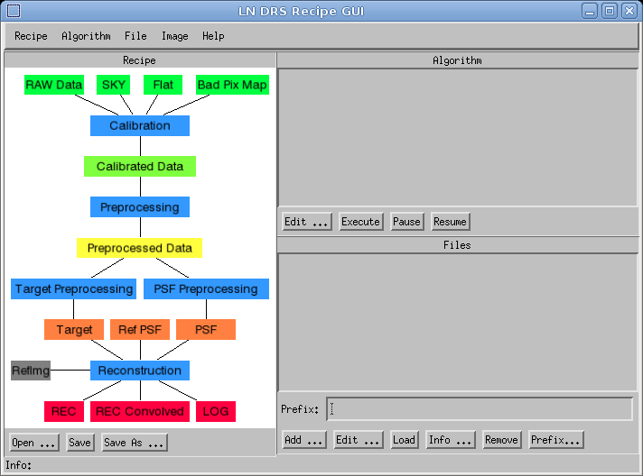
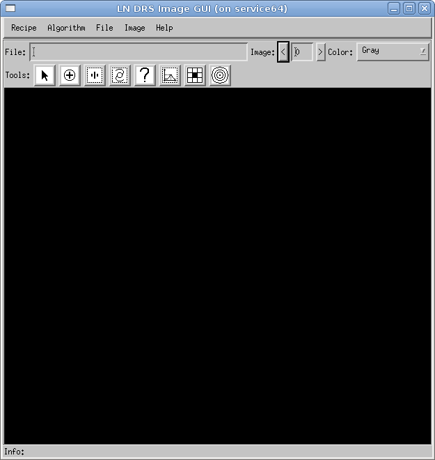
This tutorial covers only the graphical user interface, which provides functions for manipulating a parameter file and executing algorithms. A parameter file is a simple text file which contains all file names, algorithm selections and parameters necessary to execute the pipeline, which uses the raw image data and produces a reconstructed image. After starting the graphical user interface with ldrs_gui, you will see two new windows (see figure 1).

Figure 1: The main window of the LN DRS (left panel) represents the pipeline (flowchart in the left window) and provides access to the available algorithms and selected files. The image window of the LN DRS (right panel) shows loaded images and provides access to specific tools.

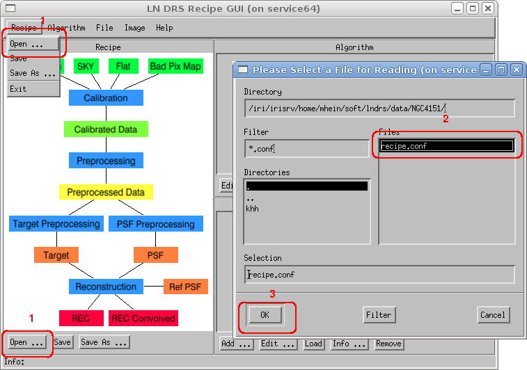
In the example NGC4151.tar.gz, a file with a parameter set is given in the file recipe.conf. In order to load these parameters into the framework, please execute the following steps (see figure 2):

1. Select the menu item Recipe/Open... from the menu bar or Open... in the main window below the flowchart.
2. In the file selection dialog box switch to your directory with the NGC4151 example (e.g. ~/lndrs/NGC4151) and select the file recipe.conf.
3. Click the Ok button in the file dialog box.

Figure 2: Window, menu and dialog box to load a parameter set.

After loading the parameter file, the elements in the flow diagram can be used to inspect file names, algorithm selections and additional parameters.

After loading the parameters, the available images can be inspected by selecting and loading a file. The example contains an artificially created sky, a flatfield and a bad pixel map. The raw file was created from simulated calibrated data by applying the inverse flatfield and adding the sky image.

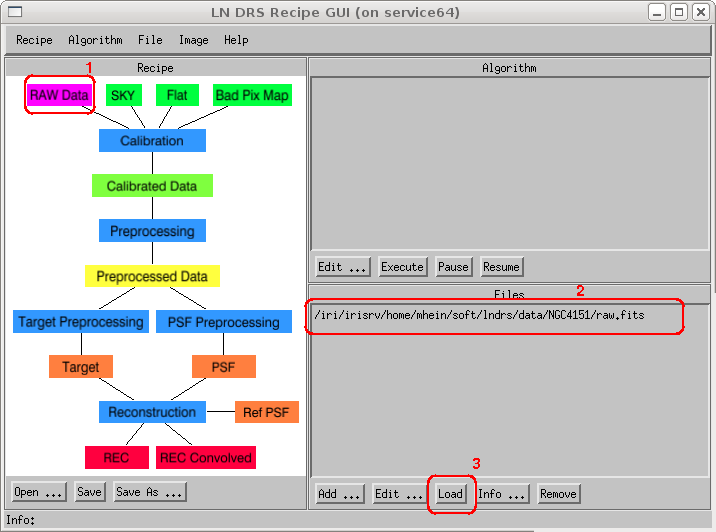
An existing file can be viewed by carrying out the following steps (see also figure 3):

1. Select the image type in the flow diagram; for example, RAW Data.
2. Select the file name in the list box in the lower left part of the main window.
3. Click on the Load button below the list box.

Figure 3: Load an existing image.

After loading a file, the contents are shown in the LN DRS Image GUI window (see figure 4). If the file contains several images (several position angles), the first image is displayed.

Figure 4: A loaded image is shown in the LN DRS Image GUI window.

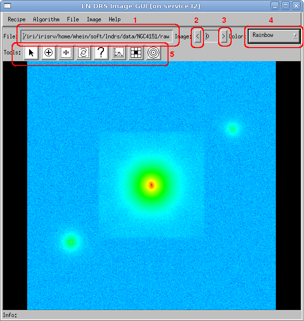This window provides the following functional interface:

1. The file name of the image currently shown in the window.
2. A mouse click on the < button switches to the preceeding image (lower image number).
3. A mouse click on the > button switches to the following image (higher image number).
4. The current color map can be switched by using this option menu.
5. These tools are necessary to parameterize the preprocessing, target preprocessing and PSF preprocessing steps.

By using the view tool (see section View Tool), the user can explore an image in more detail or get an overview.

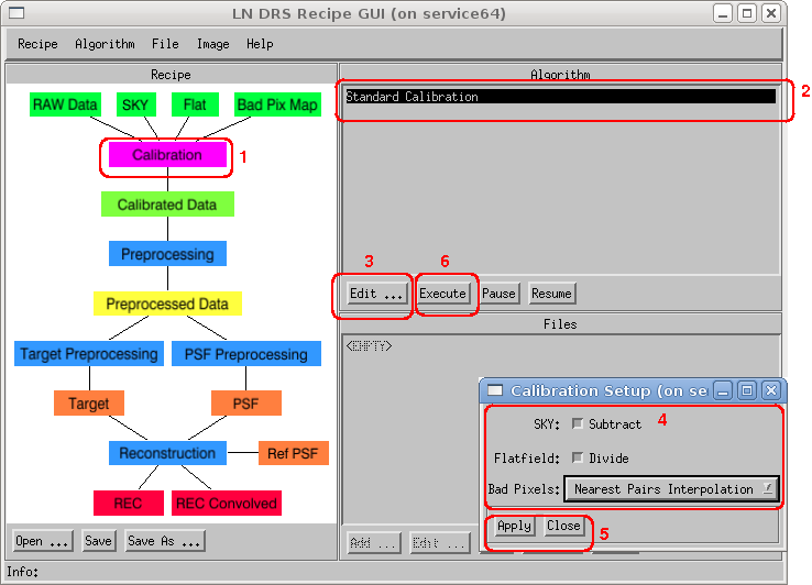
An astronomer receives the raw data, flatfield images, a valid bad pixel map and sky images from an observation. The raw images must be calibrated before further preprocessing and reconstruction can be applied. The calibration step only compensates for instrumental and detector effects. The mapping of the pixel to the sky is not changed. The steps necessary to execute a calibration are (see figure 5):

1. Select the calibration step in the flow diagram.
2. Select the specific algorithm.
3. Click the Edit button below the list box to display the algorithm-specific Calibration Setup dialog box, or double click on the algorithm name in the list box.
4. In the dialog box, set the specific parameters.
5. Click Apply after changing the parameters and on Close to close the dialog box.
6. The calibration step is executed by clicking on the Execute button below the list box.

Figure 5: Performing a calibration.

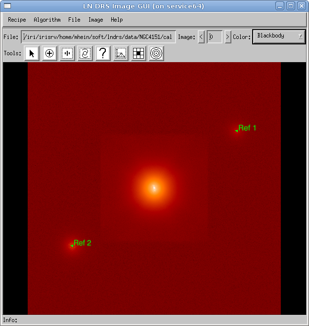
After the calibration is executed, the contents of the first calibrated file are displayed in the LN DRS Image GUI window (see figure 6).

Figure 6: Calibrated data.

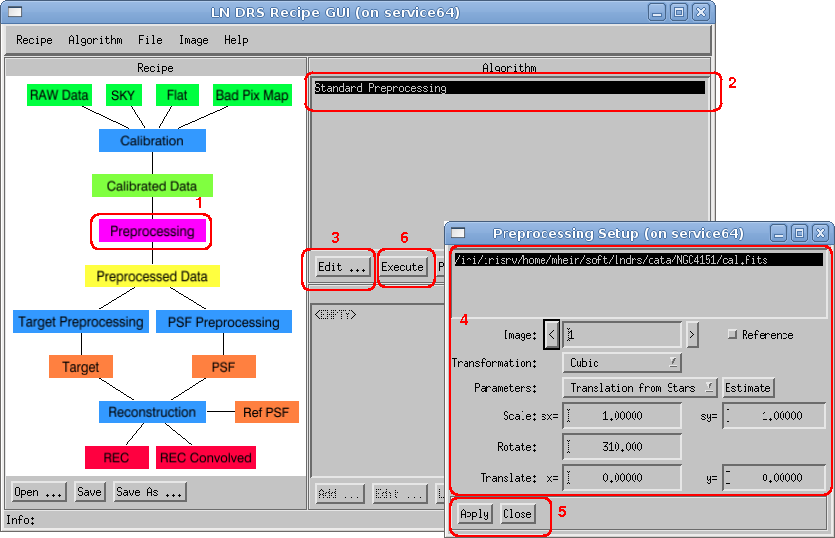
The preprocessing step changes the mapping of the calibrated images. This means that the orientation (mapping on the sky) of all images is identical after this step. The steps necessary to preprocess the calibrated data are (see figure 7):

1. Select the preprocessing step in the flow diagram.
2. Select the specific algorithm.
3. Click on the Edit button below the list box to display the algorithm-specific Preprocessing Setup dialog box.
4. In the dialog box, set the specific parameters (see section How to determine the preprocessing parameters).
5. Click on the Apply button after changing the parameters and on the Close button to close the dialog box.
6. The preprocessing step is executed by clicking on the Execute button below the list box.

Figure 7: Preprocessing.

After the data has been preprocessed, the contents of the first preprocessed file are displayed in the LN DRS Image GUI window (see figure 8). In this figure, it is obvious that at least one image is tilted compared to the original orientation in the calibrated image (see figure 6).

Figure 8: The image window shows the first preprocessed interferogram (for the first position angle).

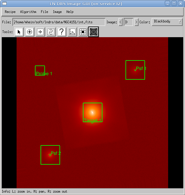In the center of the image, the target is marked with a green square and the label Target 1. Both available psf stars are marked with green squares, too (labels Psf 1 and Psf 2).

Before extracting a target from the preprocessed images, it is necessary to create a target object in the first image of each file. In the provided example, the target is already marked and ready to use. The steps necessary to define a target including sky background are described in a separate section (see section How to extract a target).

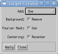
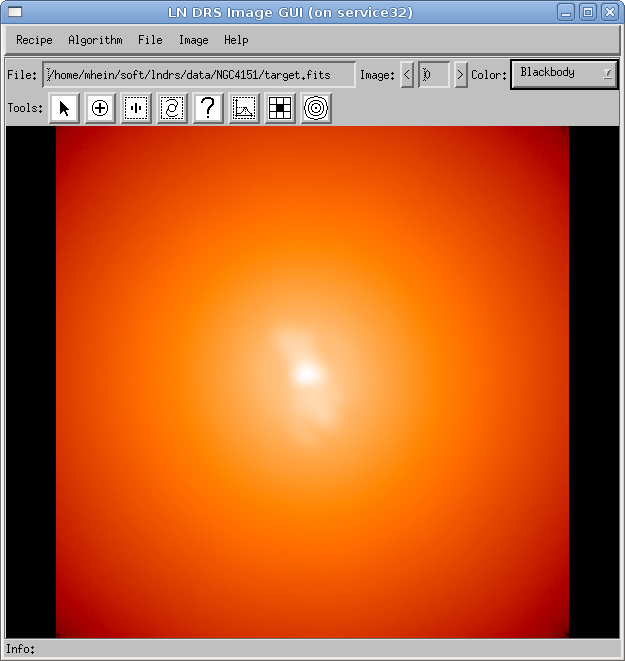
The target preprocessing is executed like the calibration or preprocessing step. The algorithm-specific dialog window is presented in figure 9 and the result is shown in figure 10.

Figure 9: The algorithm-specific target creation setup dialog.

Figure 10: The target image created from the target preprocessing step.

Before extracting a psf from the preprocessed images, a graphical representation of at least one psf star must be created in the first image of each file. In the provided example, two psf stars are already marked and ready to use.

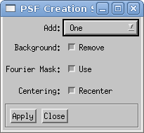
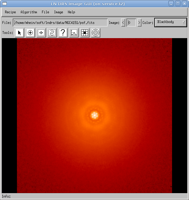
The psf preprocessing is executed like the target preprocessing step. The algorithm-specific dialog window is presented in figure 11 and the result is shown in figure 12.

Figure 11: The algorithm-specific psf creation setup dialog.

Figure 12: The psf image created from the psf preprocessing step.

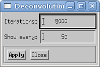
After creating the target and psf image as an input to the reconstruction step, an algorithm is selected and specific parameters are set (figure 13).

Figure 13: The algorithm-specific reconstruction setup dialog.

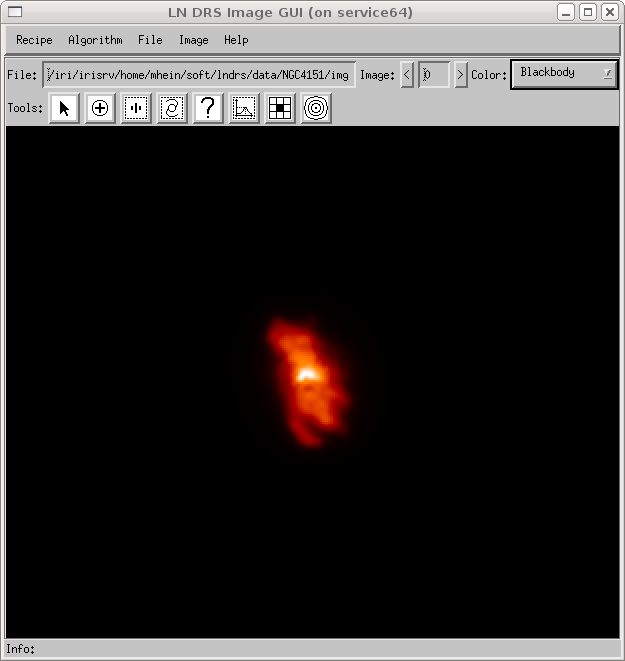
During reconstruction, intermediate results are displayed in the image GUI. It is possible to interrupt and resume or terminate a reconstruction (buttons Pause and Resume below the algorithm list box in the LN DRS Recipe GUI window (see the left panel in see figure 1). The result of the reconstruction step is automatically displayed afterward (figure 14).

Figure 14: The reconstructed target convolved with the reference psf (23m psf).