Polygons
"Without Geometry life is pointless."
In "King of Infinite Space: Donald Coxeter, the Man Who Saved Geometry", by
Siobhan Roberts.
In this site, I will be showing many geometrical models made using the Zometool system, which was developed by Steve
Baer, Clark Richert, Marc Pelletier and Paul Hildebrandt. For this reason, I will explain
some of its features that will be useful for understanding what follows.
Points, line segments, the Zometool
In Fig. 2.1, I show the standard components of the Zometool, these represent zero and
one-dimensional elements, points and line segments.
Geometry starts with geometric points, of zero
dimensions. These are represented in the Zometool by the connectors, all identical: they
have 12 Pentagonal holes, 20 Triangular holes and 30 rectangular holes, in a pattern that
is similar, but not identical, to the faces of the Rhombicosidodecahedron.
They have, therefore, an overall Icosahedral symmetry. They are normally provided in
white, as in this Figure, but the Zometool company sells them in a few colours.
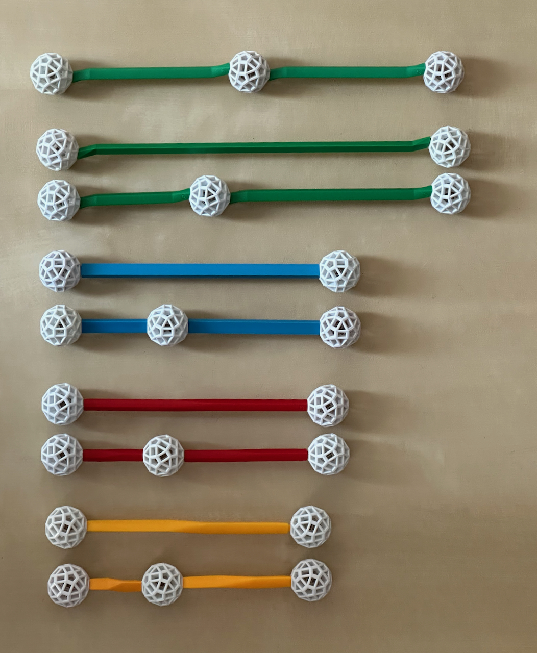
Fig. 2.1: The standard components of the Zometool. The balls are in white, the struts are
shown for sizes 0, 1 and 2 for the different colours (see explanation below for these).
In geometry, the one-dimensional objects include line segments, which in the Zometool
are represented by the struts. These are always identical at both ends:
- Those that connect to the rectangular holes of the balls are in blue (B), they align
with the 15 axes of 2-fold symmetry of the ball.
- Those that connect to the triangular holes are yellow (Y), which align with the 10
axes of 3-fold symmetry of the ball.
- Those that connect to the pentagonal holes are red (R), which align with its 6 axes of
5-fold symmetry.
- Green struts (G) also connect to the Pentagonal holes, but they have a twist at the
end to allow this.
We will keep this B, R, Y, G terminology to indicate the shapes of the struts, even when
referring to struts in non-native colours, which are also sold by the Zometool company.
The R and Y struts have a twist in the middle, which means that the balls at both ends
have always identical orientations. This means that, in any model made with the Zometool,
all balls are aligned exactly with each other!
All of these struts come in three regular sizes (n = 0, 1, 2), all shown in Fig. 2.1, with
the distance between the centres of balls attached at both ends (which we will designate
as its length) of size n being x times larger than for size n − 1 (we
will calculate this number x soon). This geometric progression means that any model
built in a size could in principle be built in a smaller or larger size. Red struts also
have a very short (00) size. Green struts also come in half-sizes (HG), two HG2 struts are
shown right at the top of the Figure. Size 3 struts were made by the Zometool company in
the early days, but they have been discontinued, and for that reason they are a bit harder
to find. I buy them mostly on eBay.
To calculate the lengths of these struts, we will now define the length of the B1 strut as
the unit of measurement. Given the geometric progression mentioned above, the B0 strut has
length 1/x and the B2 strut has length x.
Fig. 2.1 shows a very important feature of the system: size 2 struts are as long as the
sum of the lengths of struts with sizes 0 and 1:
x = 1 + 1/x (a)
Multiplying both sides by x and moving them to the left, we obtain a simple
quadratic equation:
x2 − x − 1 = 0 (b)
Using the quadratic
formula, we see that there is a single positive solution to this equation:
x = (√ 5 + 1) / 2 = 1.618 033 988 749 894 848 204 586 834 365...,
which is the Golden
ratio, φ. The the other solution to eq. (a) is Φ = −(√ 5
− 1)/2. From equations (a) and (b), we derive:
1 / φ = φ − 1 = − Φ = 0.618 033 988 749 894 848 204 586 834 365... (c)
φ2 = φ + 1 = ( √5 + 3 ) / 2 = 2.618 033 988 749 894 848 204 586 834 365.... (d),
these are the lengths of the B0 and B3 struts. Equation (d) implies φ = √(φ +
1), we can also use it to calculate all powers of φ (lengths of B4, B5, B6, B7,...):
φ3 = 2 φ + 1 = ( 2 √5 + 4 ) / 2 = 4.236 067 977 499 789 696 409 173 668 731...
φ4 = 3 φ + 2 = ( 3 √5 + 7 ) / 2 = 6.854 101 966 249 684 544 613 760 503 096...
φ5 = 5 φ + 3 = ( 5 √5 + 11 ) / 2 = 11.090 169 943 749 474 241 022 934 171 828...
φ6 = 8 φ + 5 = ( 8 √5 + 18 ) / 2 = 17.944 271 909 999 158 785 636 694 674 925...,
which merely extends what Fig. 2.1 is showing, that each term in the series is the sum of
the two previous ones. A consequence of this is the simple expressions in the second
column, which imply that any large B strut size can be built by adding as many smaller
B1 (unit) and B2 (φ) struts as indicated by the coefficients in boldface.
These coefficients necessarily grow in the same way: each new coefficient (Fn +
1) is the sum of the two previous coefficients, Fn and Fn −
1. Because this sequence started with F0 = 0 and F1 = 1, these
coefficients are the famous Fibonacci numbers. Note that
the unit coefficients are one position behind in the sequence relative to the φ
coefficients, therefore they can be written for n > 0 as:
φn = Fn φ + Fn − 1 = ( Fn √5 + Ln) / 2, (e)
where Ln = Fn + 2 Fn − 1 are the coefficients in
italic, the Lucas
numbers, defined in the same way as the Fibonacci series, the difference being
L0 = 2. Using eqs. (c) and (d), we can calculate the negative powers of φ
(lengths of B−1, B−2, B−3, B−4, B−5, ...):
φ−2 = − 1 φ + 2 = ( − 1 √5 + 3 ) / 2 = 0.381 966 011 250 105 151 795 413 165 634...
φ−3 = + 2 φ − 3 = ( + 2 √5 − 4 ) / 2 = 0.236 067 977 499 789 696 409 173 668 731...
φ−4 = − 3 φ + 5 = ( − 3 √5 + 7 ) / 2 = 0.145 898 033 750 315 455 386 239 496 903...
φ−5 = + 5 φ − 8 = ( + 5 √5 − 11 ) / 2 = 0.090 169 943 749 474 241 022 934 171 828...
φ−6 = − 8 φ + 13 = ( −8 √5 + 18 ) / 2 = 0.055 728 090 000 841 214 363 305 325 074...
As for positive powers, each power and its associated coefficients is the sum of the two
previous powers and their associated coefficients. The coefficients in boldface and italic
are again the Fibonacci and Lucas numbers, only that their signs alternate (these are the
Fibonacci and Lucas
sequences extended to negative integers) and the unit coefficients in boldface are one
position ahead in the Fibonacci sequence relative to the φ coefficients. Thus, for n >
− 1:
(− φ)− n = Φn = − Fn φ + Fn + 1 = (− Fn √5 + Ln) / 2, (f)
where we used the relation Ln = − Fn + 2 Fn + 1.
In the limit of very large values of n, Φn converges to zero and
φ = Fn + 1 / Fn, Ln / Fn = √5.
The convergence of the ratio of two successive terms of the Fibonacci sequence to φ,
which was first demonstrated by Kepler, implies that the same happens for all sequences of
positive reals where each term is the sum of the two previous ones, like the Lucas
numbers.
***
As an aside, these powers of φ yield, in a simple way, many exact relations between
φ, the Fibonacci and Lucas numbers. For a few examples, adding (f) to (e), we obtain
an equation that allows the calculation of the Lucas numbers without the need to know all
previous terms in the sequence. Subtracting (f) from (e), we obtain a similar equation for
the Fibonacci numbers, Binet's
formula:
φn + Φn = Fn − 1 + Fn + 1 = Ln, (φn − Φn) / √5 = Fn. (g)
The first equation implies that for |Φn| < 0.5 (i.e., n > 1), all
φn round to Lucas numbers, as we can see for the positive powers of φ
above by comparing the coefficient in italic and the numerical value. As n increases, the
difference quickly becomes extremely small. Multiplying (e) and (f), we obtain
φn Φn = (− 1)n = (Fn φ + Fn − 1)( − Fn φ + Fn + 1) = ( Fn √5 + Ln)( − Fn √5 + Ln) / 4, (h)
from the third and fourth expressions, we obtain beautiful relations for the squares of
the Fibonacci and Lucas numbers:
Fn2 = Fn − 1 Fn + 1 − (− 1)n,
Ln2 = 5 Fn2 + 4(− 1)n = 5 Fn − 1 Fn + 1 − (− 1)n. (i)
The first equation is the famous Cassini
identity, which was, however, already known to Kepler. If we multiply the two
equations (g), or if we square them, we obtain respectively
F2n = Ln Fn and L2n = Ln2 − 2 (− 1)n = 5 Fn2 + 2 (− 1)n, (j)
where the first equality of eq. (h) was used to derive the second set of equations.
Equations (g), (i) and (j) are valid for all integer values of n.
***
Apart from the scalability, the reason why φ is important for polytopes has to do with
the fact that it is the ratio of the length of the diagonal of the regular pentagon
(L) to the length of its side (ℓ). The proof below is described in Livio
(2002), but it is originally in Euclid's Elements. It decomposes the Pentagon into
three isosceles
triangles: one Golden triangle in
the middle and two Golden
gnomons on the sides.
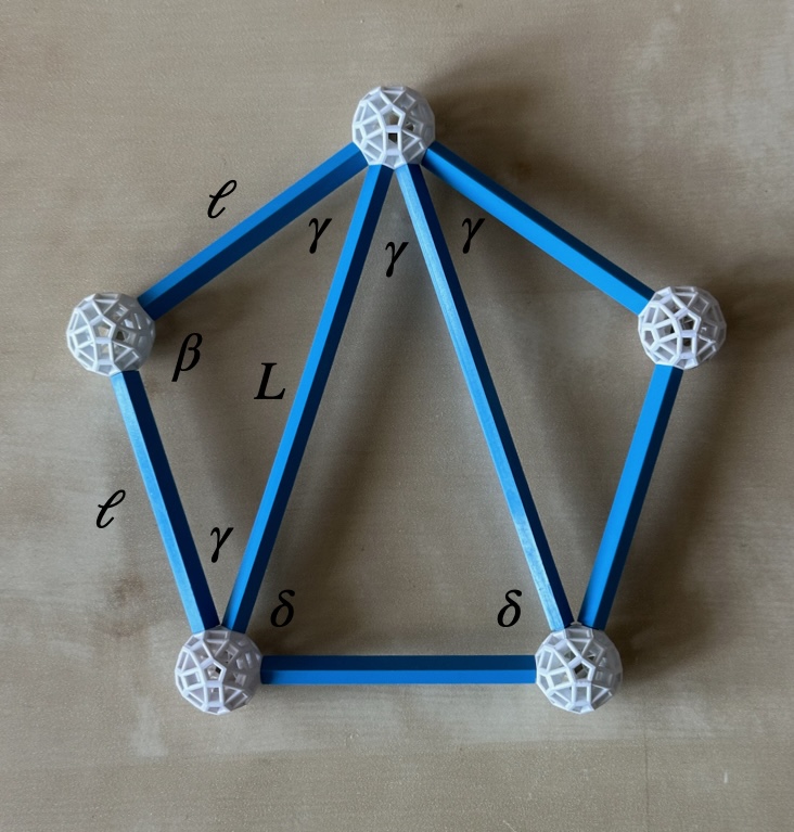
Fig. 2.1a: The outside figure is a Pentagon, here built with B1 struts. This can be
decomposed into a Golden triangle (at the centre) and two Golden gnomons on the left and
right. The lines separating the inner Triangles (built here with B2 struts) are the
diagonals of the Pentagon.
The larger angle of the Golden gnomon (β) is the inner angle at the vertex of the
Pentagon, which as we'll see later is 108 degrees. Given that the two small sides of the
Golden gnomon are identical (they are two consecutive sides of the Pentagon), its two
remaining angles (γ) must also be identical. The sum of the inner angles of any
triangle must be 180
degrees, so from β + γ + γ = 180, we obtain γ = 36 degrees.
Since the Golden gnomon on the right also has angle γ at this vertex, the small
angle of the Golden triangle is 108 − 36 − 36 = 36 degrees = γ; i.e.,
the diagonals of the Pentagon trisect its inner angle. Since
the two identical angles of the Golden triangle (δ) plus γ must add up to 180
degrees, we obtain δ = 72 degrees.
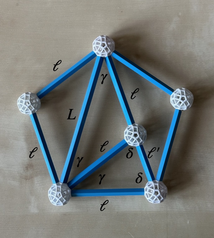
Fig. 2.1b: Bisecting one of the C angles of the Golden Triangle, we obtain a Golden gnomon
and a smaller Golden triangle, as shown below.
In Fig. 2.1b, we bisect one of the δ angles of the central Golden triangle, thus
making two angles of 36 degrees = γ. This bisection divides the Golden triangle
into two smaller triangles. For one of them, the smaller angles are both γ = 36
degrees, so it is a Golden gnomon.
The smaller triangle is very interesting: it has an angle given by γ, and from Fig.
2.1b we already knew that it has another angle given by δ, so the remaining angle
must be 180 − 72 − 36 degrees = 72 degrees = δ. Thus the smaller
triangle is another Golden triangle! Furthermore, since this and the previous Golden
gnomon are isosceles triangles, and one of the equal sides is common, all their equal
sides have length ℓ. To summarise, bisecting one of the larger angles of a Golden
triangle, we decompose it into a Golden gnomon and a smaller Golden triangle.
The ratios between the larger and smaller sides of the large and small Golden triangles
must be identical:
L / ℓ = ℓ / ℓ'
where ℓ' is the smaller side of the smaller Golden triangle. However, we see from Fig.
2.1b that L = ℓ + ℓ', thus,
(ℓ + ℓ') / ℓ = ℓ / ℓ',
1 + ℓ' / ℓ = ℓ / ℓ'.
If we replace ℓ / ℓ' by x we obtain eq. (a), which has the same numerical
solution, φ. Thus φ is L / ℓ, the ratio of the diagonal of a Pentagon
to its side, the ratio between the sides of the Golden triangle, the ratio of the sides of
the Golden gnomon (hence their names) and the ratio of sizes between a Golden triangle and
the smaller Golden triangle within it. This is, of course, the reason why we can represent
Figs. 2.1a and b with B0, B1 and B2 struts. The full implications of this will become
clear in Figs. 2.6a and b.
***
We now calculate the lengths of the other struts. For this, we will apply the Pythagorean
theorem to estimate the lengths of the diagonals of a sequence of rectangles.
Before that, we note that their lengths are irrational numbers. The proof
that the length of the diagonal of a Square or unit edge (√2) is irrational is very famous,
having presumably been found by the Pythagoreans. However, this can be made much simpler
and more general. If for an integer n √n were rational but not an integer, then it
could be written as an irreducible fraction p/q, i.e., where p and q are integers with no
common prime factors. However, this would imply that, after squaring this equality
n = p2/q2
the fraction on the right is also irreducible: it has the same set of prime factors on the
numerator and denominator as p/q. Therefore n cannot be an integer, contradicting the
assumption. n can only be an integer if q = 1, in which case it is a perfect square. The
same argument is true for higher powers: apart from perfect cubes, all integers have
irrational cubic roots, and so ad infinitum. This implies that φ is also irrational,
because it is a sum of a rational and irrational number, √5.
Despite being irrational, the lengths of these diagonals are by definition constructible numbers
because the diagonals can be constructed with a compass and
straightedge in a finite number of steps. We will now show these constructions:
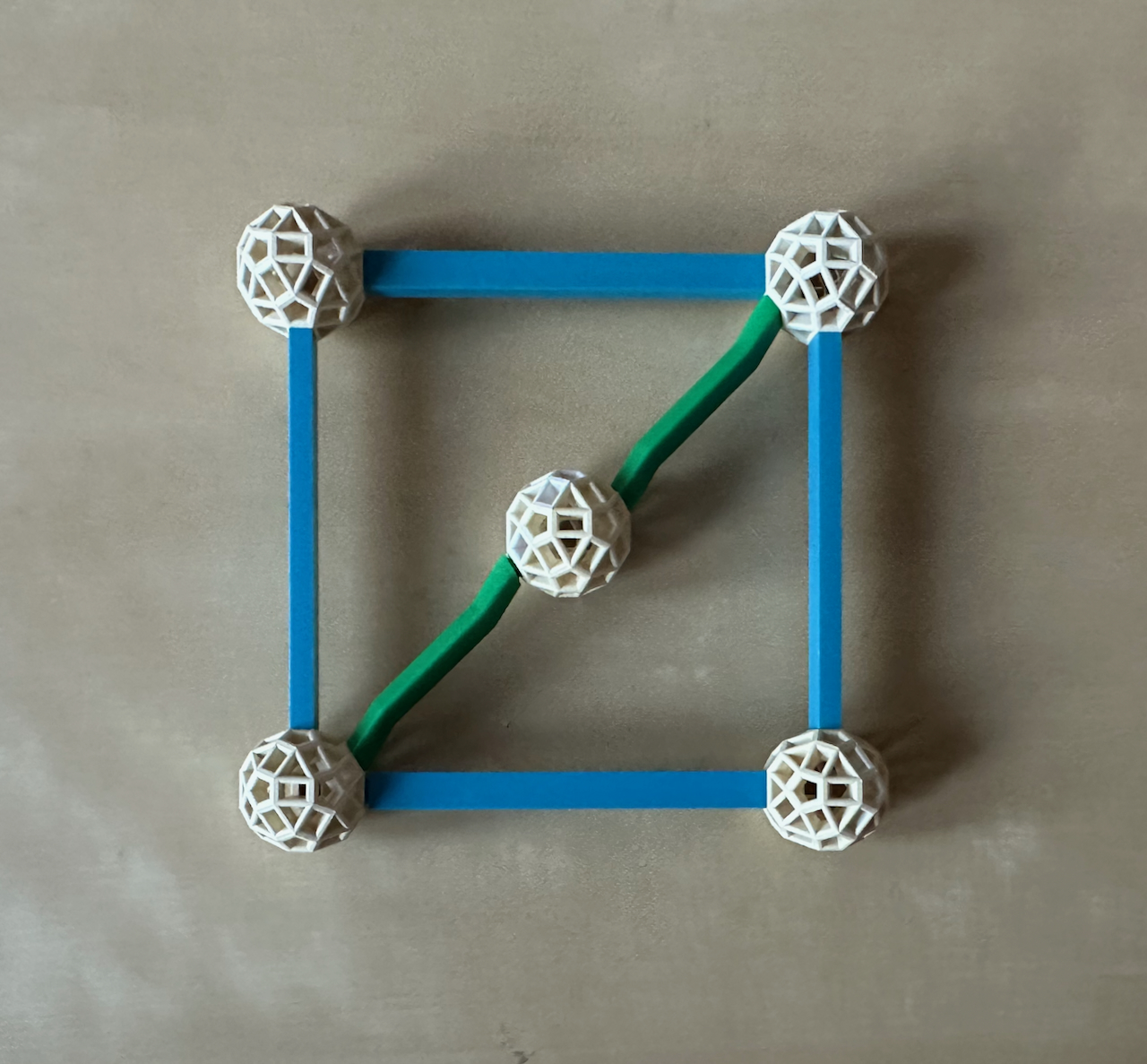
Fig. 2.2a: A Square built with B1 struts. Two HG1 struts represent the diagonal, they add
to the length of a G1 strut.
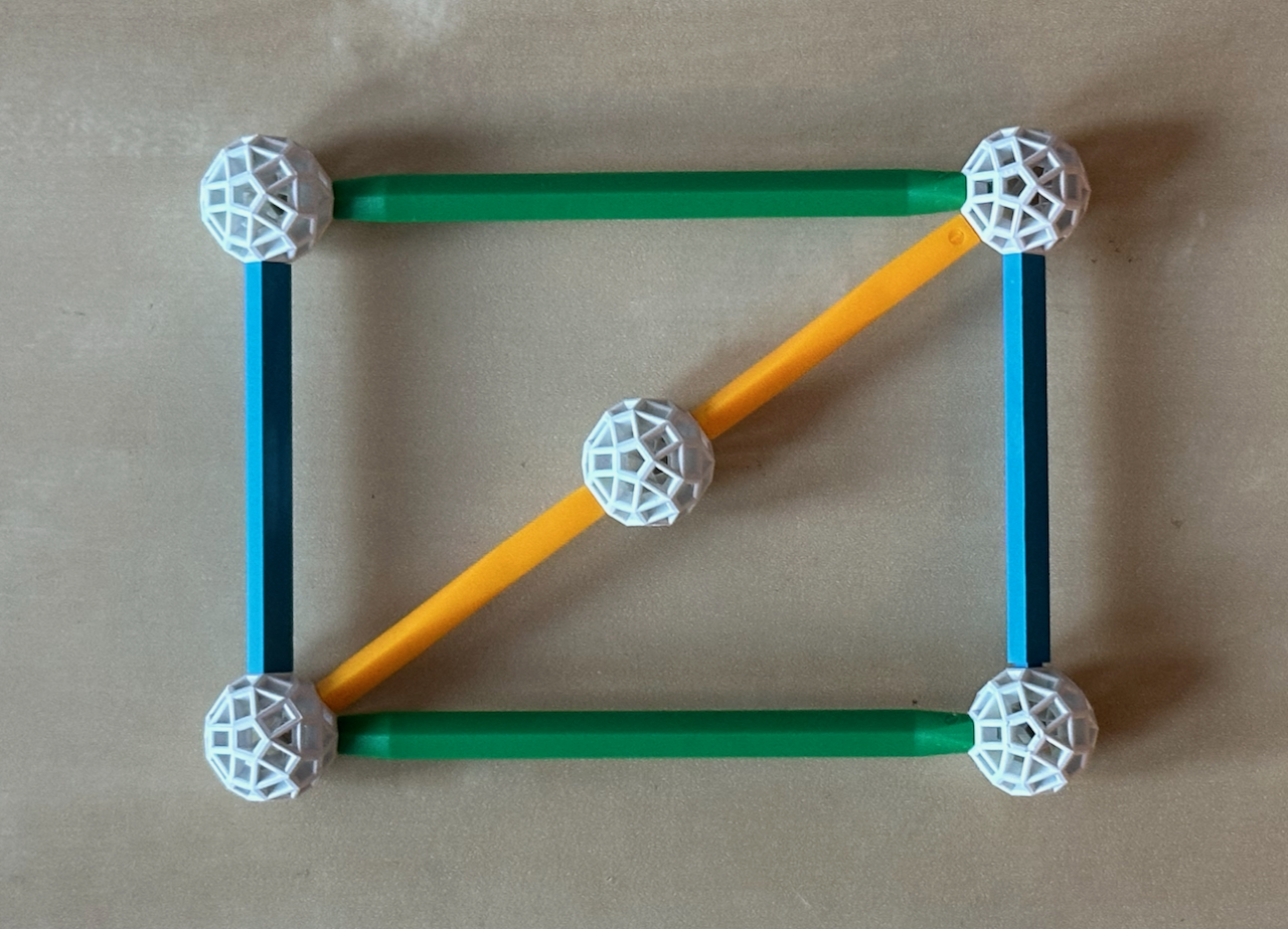
Fig. 2.2b: A Rectangle
built with B1 and G1 struts, the latter is the diagonal of the Square in Fig. 2.2a.
The Square in Fig. 2.2a
has two B1 struts as sides, both with length 1. Thus, its diagonal is given by h = √
(1 + 1) = 1.414 213 562... This is the length of a G1 strut. The two HG1 struts shown have
half this length, h/2 = √2 / 2 = 0.707 106 781... For other HG sizes, multiply by the
different powers of φ.
The rectangle in Fig. 2.2b has B1 and G1 struts as sides, with lengths of 1 and √2.
Thus, h = √ (1 + 2) = 1.733 050 807... The two Y1 struts shown have h/2 = √3 / 2
= 0.866 025 403... For other Y sizes, multiply by the different powers of φ. Because
the diagonal is represented by yellow struts, I call this a Yellow rectangle. This has the
proportions of A4 paper,
which are kept when cut or folded in half withdways.
Mathematically, this process can go on forever, obtaining the lengths of all square roots,
and building the Spiral of Theodorus. The next
square root - of length 2 - is shown in Fig. 4.4a. In this page we continue instead with
the Golden
rectangle. In Figure 2.2c, we construct it from a Square with unit edge length (B1) on
the left.
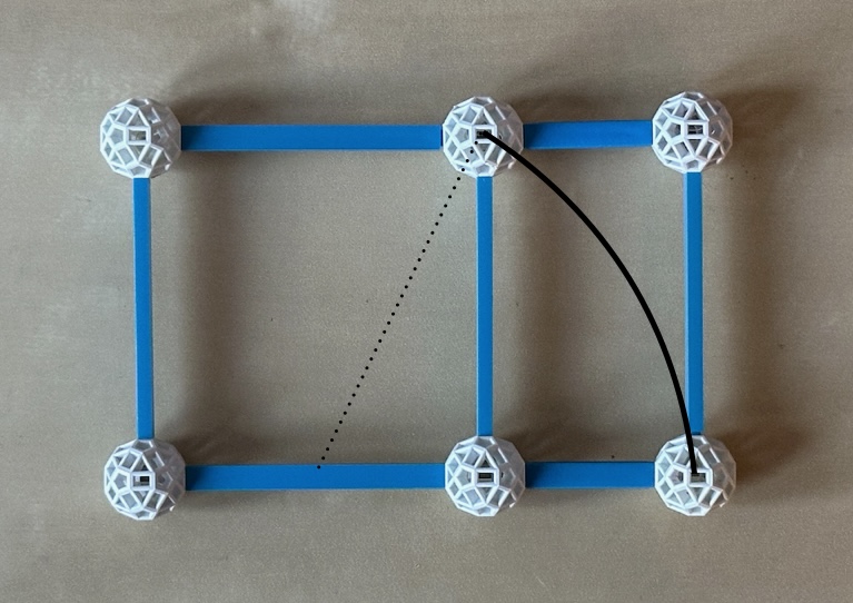
Fig. 2.2c: Construction of a Golden rectange from a Square.
We then mark the middle of the lower edge, open the compass to the upper right corner,
covering a distance of √((1/2)2 + 1) = √5/2. Then mark that distance
on the horizontal axis. The width of the full figure is now 1/2 + √5/2 = φ, in
this case the length of a B2 strut. The length added to the side of the original Square is
√5/2 − 1/2 = φ − 1 = 1/φ. From this, we see that one of the
properties of Golden rectangles is that subtracting a Square (on the left), we obtain a
smaller, vertical Golden rectangle (on the right). This property is analogous to the
division of Golden triangles into Golden gnomons and smaller Golden triangles.
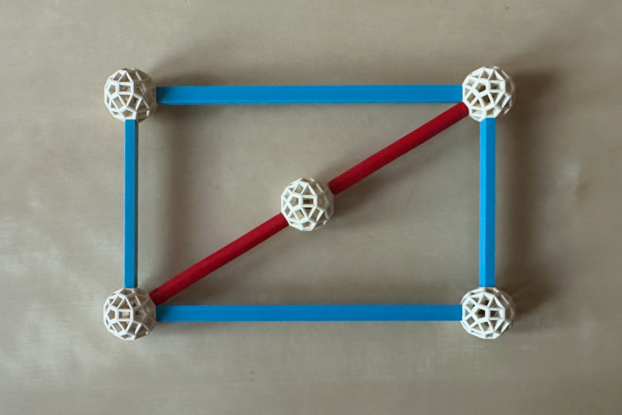
Fig. 2.2d: The diagonal of a Golden rectangle can be covered with two R1 struts.
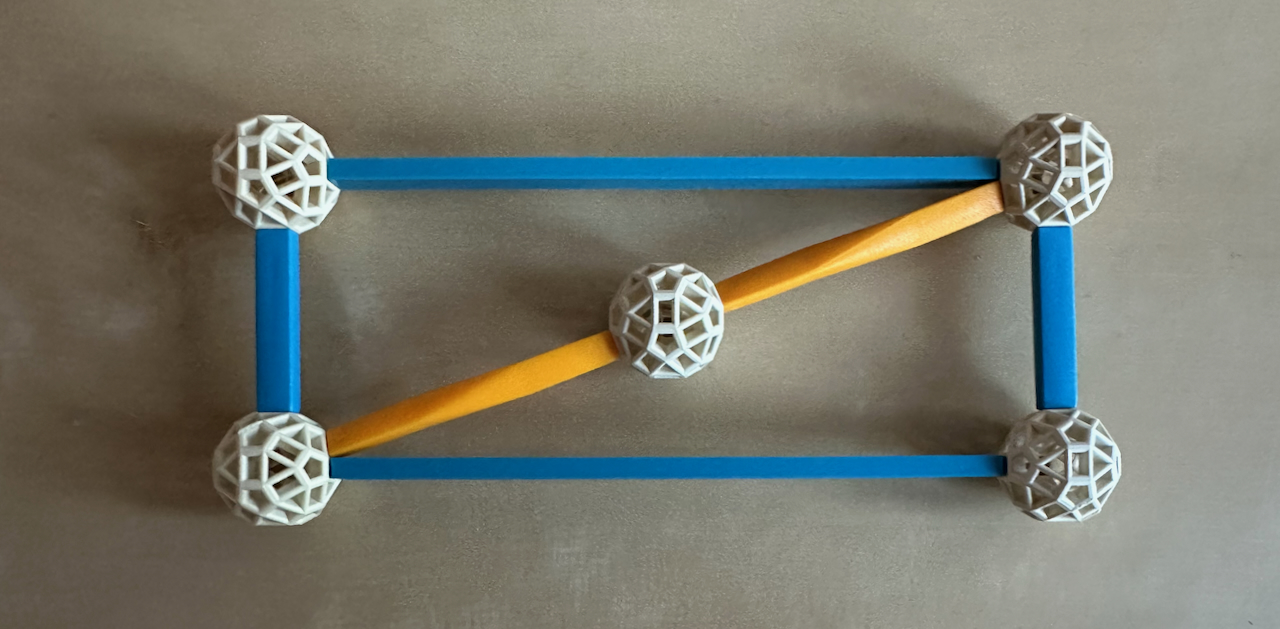
Fig. 2.2e: A Rectangle built with B0 and B2 struts. Two Y1 sruts represent the diagonal.
The Golden rectangle in Fig. 2.2d has B1 and B2 struts as sides, with lengths of 1 and
φ. Thus, h = √(1 + φ2) = √(2 + φ) = √ ((5 +
√5) / 2) = 1.902 113 032... The two R1 struts shown have h/2 = √ ((5 + √5)
/ 8) = 0.951 056 516... For other R sizes, multiply by the different powers of φ.
Finally, the rectangle in Fig. 2.2e has B0 and B2 struts as sides, with lengths of 1/φ
and φ. Thus:
h = √(φ2 + φ−2) = √L2 = √3 (k).
where we used the first (g) equation. The result is the same as in Fig. 2.2b, which means
that the diagonal can also be covered by two Y1 struts, as we see in Fig. 2.2e! For this
reason, I call this the Long yellow rectangle. Its area is given by φ × 1/φ
= 1, i.e., the same as the Square in Fig. 2.2a. See model related to the Golden and Long
yellow rectangles in Fig. 4.4b.
These lengths will be useful through the whole site, we will use them below to study the
regular polygons. For many more models explaining the properties of the Zometool, see Hart
(2000).
Zomable polygons
There are many types of two-dimensional figures. In what follows, we will concentrate on
polygons. We have already
depicted a few polygons above (triangles, rectangles, the Square and the Pentagon): they
are finite regions of 2-D Euclidean space* bound by at
least 3 straight line segments, or sides; these sides meet in
pairs, in angles different from 0 and 180 degrees, at an identical number of vertices. In
what follows, we regard all polygons and generally polytopes as closed sets, which means that their
surface elements (henceforth "elements") are also part of them.
* This is the traditional definition of a polygon. We will not consider here apeirogons, skew polygons, or complex polygons.
A regular polygon
(henceforth Polygons) is isogonal and isotoxal. This means that not only
are the elements identical (sides of the same length, edge-vertex-edge angles - the "inner
angles" - identical), but the polygon looks the same from all elements of a particular
type. It follows from this that the polygon has a well defined centre and that all
elements of a particular type are equidistant from it.
The names of polygons generally denote the number of sides, which is the the same as the
number of vertices; for instance the name ``pentagon'' means ``five sides'' in Greek. In
this site we use capitalised polygon names to refer to their regular forms. The non-Greek
names are the triangle, which refers to the three inner angles, and the quadrilaterals: Isogonal
quadrilaterals are called rectangles, isotoxal quadrilaterals are called rhombuses; isogonal and isotoxal are
regular, the Square.
The polygons shown above can be built with the Zometool, i.e., they are Zomable. We
now expand this, depicting other Zomable Polygons and special rhombuses. Because the
Zometool parts represent only points (with the balls) and line segments (with the struts),
it only represents the surface elements of the polygons, the vertices and the sides. We
also display a strut connecting the vertex of the polygon to its center if this can be
represented with the Zometool, which tells us something about its metric properties. This
study will be useful for the latter study of figures in higher dimensions, also for
showcasing the capabilities of the Zometool system.
All Zomable polygons depicted in this page, including all regular polygons, are constructible,
i.e., they can be built with a compass and straightedge. However, this is not the case for
most polygons.
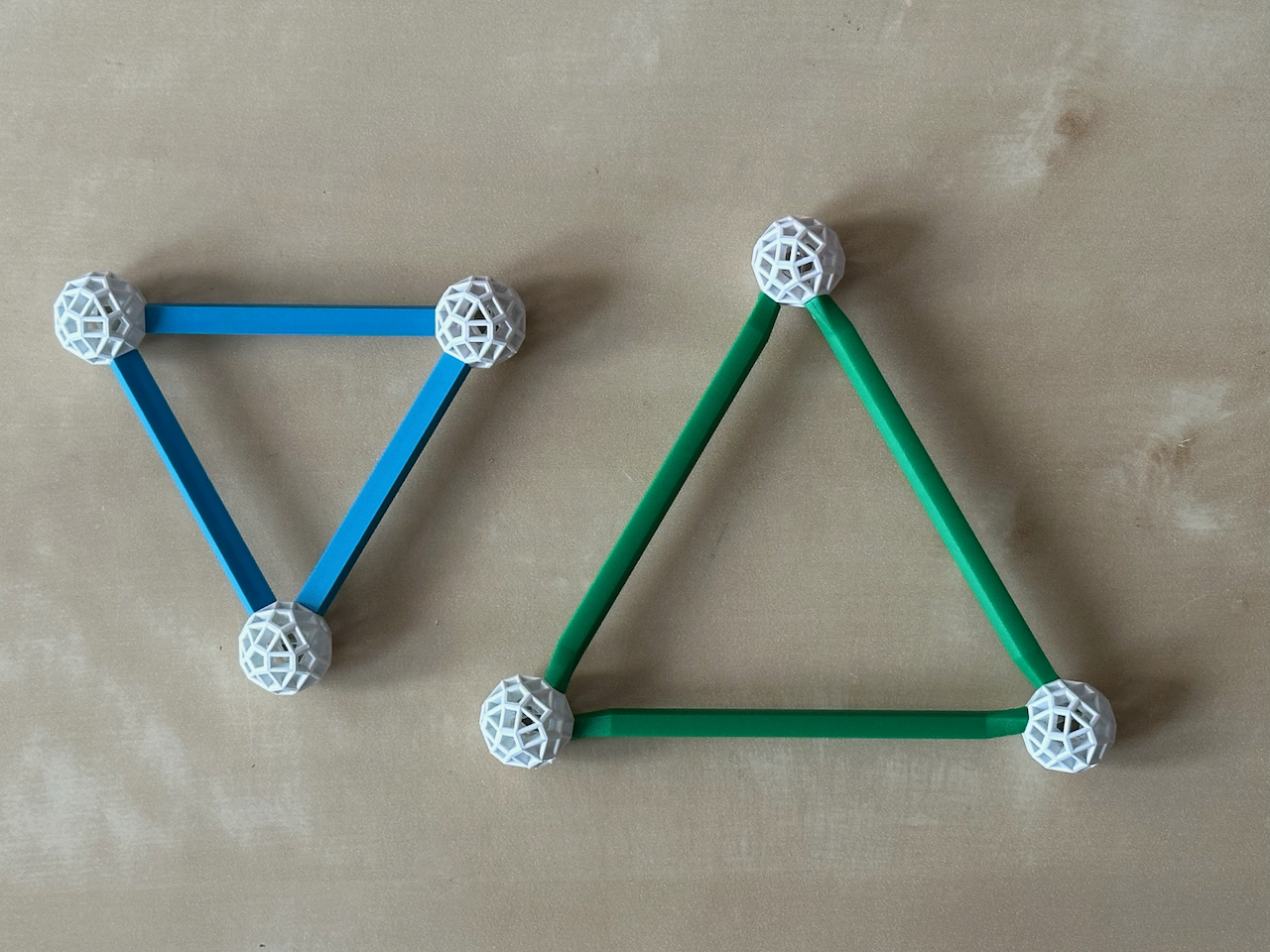
Fig. 2.3a: Triangles can be huilt with
B and G struts.
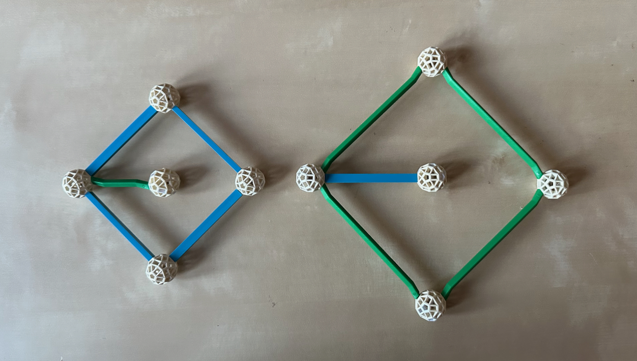
Fig. 2.3b: Squares, which we have already seen built with B struts (fig. 2.2a), can also
be built with G struts. Additionally, we can also see that the distance from the centre of
the square to a vertex can be represented by struts of the other colour.
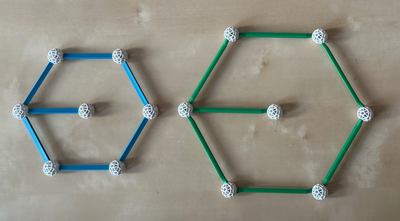
Fig. 2.3c: Hexagons can be built
with B and G struts; this is a consequence of this also being true for Triangles, six of
which can fill the Hexagon.
In Fig. 2.3c, the distance from the centre of the Hexagon to a vertex can be represented
by struts of the same colour and length as its edges. This means that the distance of the
centre to the vertex is the same as its side, i.e., the Hexagon is radially
equilateral. It is the only Polygon with this characteristic.
Heptagons, Octagons and Nonagons are
not Zomable. The Heptagon and Nonagon are non-constructible, the simplest such figures.
The Octagon is easily constructible, but the fact that it is not Zomable will have
important implications later. However, there is one last Zomable convex Polygon, the Decagon;
which like the Pentagon (Figs. 2.1a, b) can only be built with B struts.
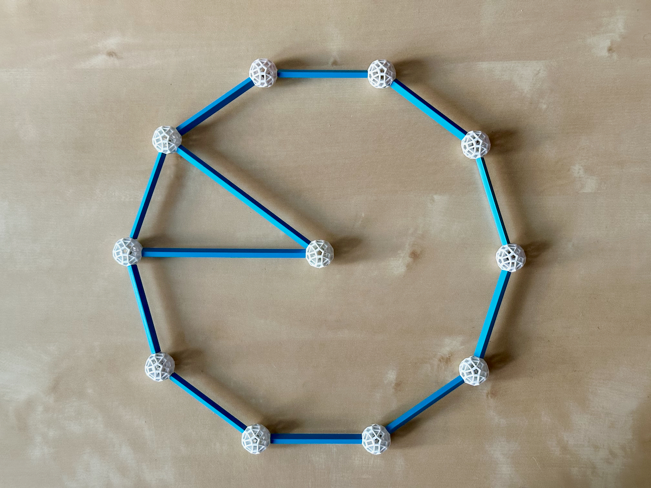
Fig. 2.3d: Like the Pentagon, the Decagon can only be built with B struts.
In Fig. 2.3d, since the angle subtended by each side at the centre is 360 / 10 = 36
degrees, we can decompose the Decagon into ten Golden triangles radiating from the centre
(one of them represented in the figure). Thus, the distance from the centre to a vertex is
the same as the diagonal of a Pentagon of the same side (Figs. 2.1a, b), φ times
longer than the sides, and thus representable with a 1 size larger B strut.
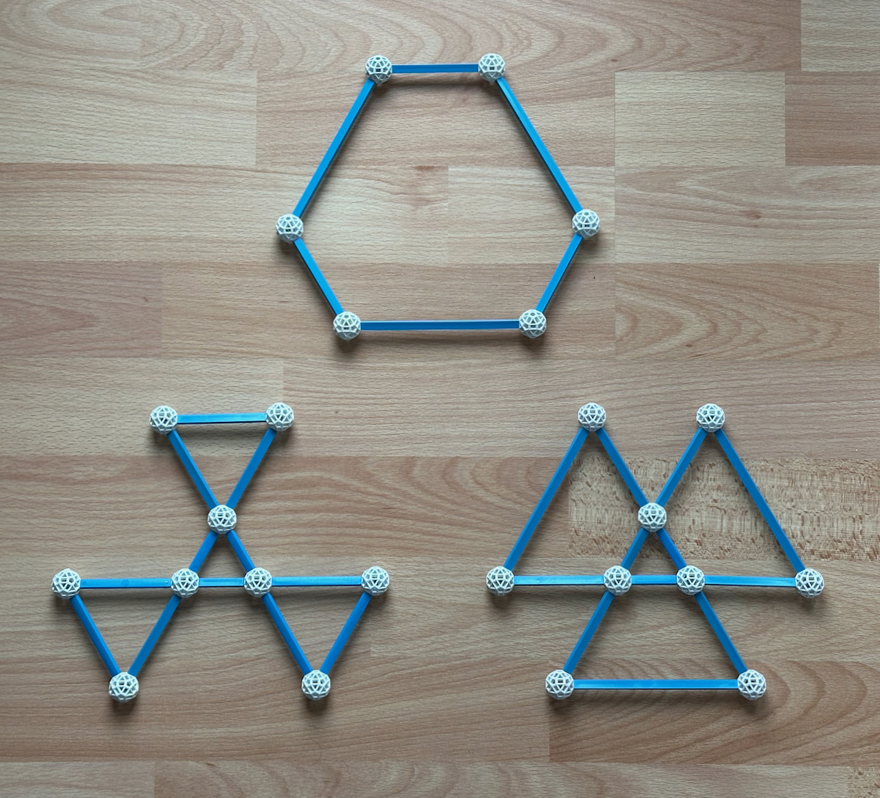
Fig. 2.3e: The ditrigonal hexagons. These three hexagons share the same vertex
arrangement, all of them are isogonal, but have edges with two lengths.
Of course, with Zometool we can represent many irregular polygons. In Fig. 2.3e, I show
three special cases of irregular hexagons with 3-fold symmetry, the ditrigonal hexagons:
these are, on top, the ditrigon, on lower left the propeller
tripod and on lower right the tripod. The three share the same
vertex arrangement and are all isogonal (within each polygon, they have the same angle and
side lengths at each vertex: 120 degrees for the ditrigon, 60 degrees for the tripods),
but their edges come in two different lengths, i.e., they are not isotoxal. The lengths of
the edges are: 1 and 1/φ for the ditrigon, φ and 1/φ for the propeller tripod
and φ and 1 for the tripod. The tripods are non-convex; furthermore, their long edges
cross each other (each one crosses the other two). This makes them star polygons. These crossing points
are false vertices (represented by the inner balls), because no edge ends there.
Geometric relations
To continue, we will now discuss several geometric transformations between polygons, which
will be useful to understand all polytopes in general, they will also give us an
opportunity to discuss regular star polygons and several special non-regular
quadrilaterals.
Duality: If
polygons A and B are dual, then to a vertex of A corresponds an edge of B. This is a
reciprocal relation, so to each vertex of B corresponds an edge of A. Two dual polygons
have the same symmetry.
We now show examples of the rectangle-rhombus
duality: To the isogonal Rectangles correspond the isotoxal rhombuses; to the
alternate side lengths of the rectangles correspond the alternate angles of the rhombuses.
The rhombuses touch the rectangles at right angles with a line from the vertex of the
rectangle to the centre; this is known as the ``
Dorman Luke'' construction, which can be used in any case where a polygon has a
centre. In the figues below, we demonstrate this by drawing a special circle, which
touches all the vertices of the rectangles (i.e, this circle circumscribes the rectangles)
and tangentially touches all the sides of the rhombuses (i.e., this circle is inscribed in
the rhombuses).
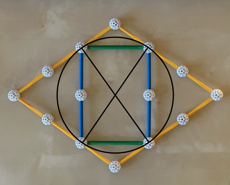
Fig. 2.4a: The Yellow rectangle and its dual, the Yellow rhombus. To achieve this
particular construction, we had to glue two yellow rectangles by their longer sides,
obtaining a larger Yellow rectangle.
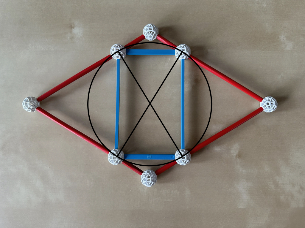
Fig. 2.4b: The Golden rectangle and its dual, the Golden rhombus.
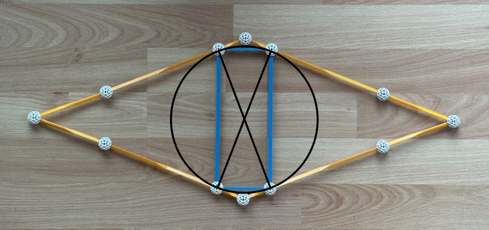
Fig. 2.4c: The Long yellow rectangle and its dual, the Long yellow rhombus.
Thus, the duals of the Yellow, Golden and Long Yellow rectangles in Figs. 2.2b, d and e
are the Yellow, Golden and Long yellow rhombuses
in Figs. 2.4a, b and c.
The dual of the isogonal ditrigonal hexagons in Fig. 2.3e is a set of isotoxal hexagons,
also possessing 3-fold symmetry, the triambuses. These are, however, not
Zomable.
If a polygon is regular, its dual is of the same kind, but rotated by 180 deg / n, where n
is the number of sides of the Polygons (see Fig. 2.4d). Thus, unlike most other types of
polygons, regular polygons are self-dual.
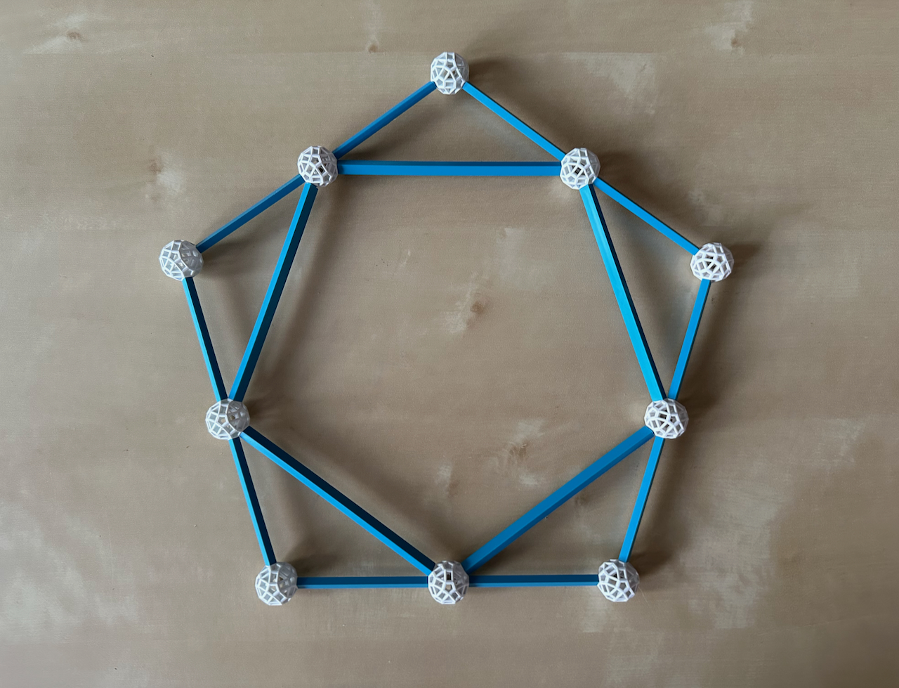
Fig. 2.4d: The dual of a regular Polygon like the Pentagon is of the same kind: another
Pentagon. The inner and outer Pentagons are duals of each other.
Rectification:
Rectification consists of marking the mid-points of the sides of a polygon and cutting off
the vertices at those points. This results in a new polygon, which is the rectification
of the first one.
In the case of a Polygon, the rectification is of the same kind, but rotated by 180 deg /
n, where n is the number of sides of the Polygons, and smaller. In Fig. 2.4d, the inner
Pentagon, which is the dual of the outer pentagon, is also its rectification.
However, the rectification is not the same as a duality. If we rectify Yellow, Golden or
Long yellow rhombuses, we obtain again Yellow, Golden or Long yellow rectangles, but in an
orthogonal direction to that in Figs. 2.4a, b and c. In the next Figures, we see that the
Rhombic diagonals are in the same proportions as the sides of the resulting rectangles,
but twice as long, as shown later in Fig. 4.9. Thus, all struts of the rectangles in Figs.
2.5a, b and c are necessary to trace the diagonals of their respective rhombuses.
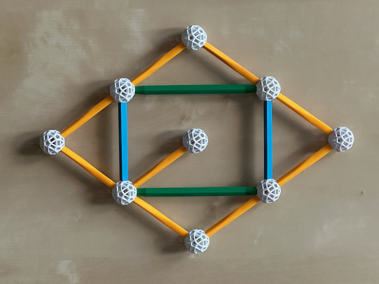
Fig. 2.5a: The rectification of a yellow rhombus is a Yellow rectangle.
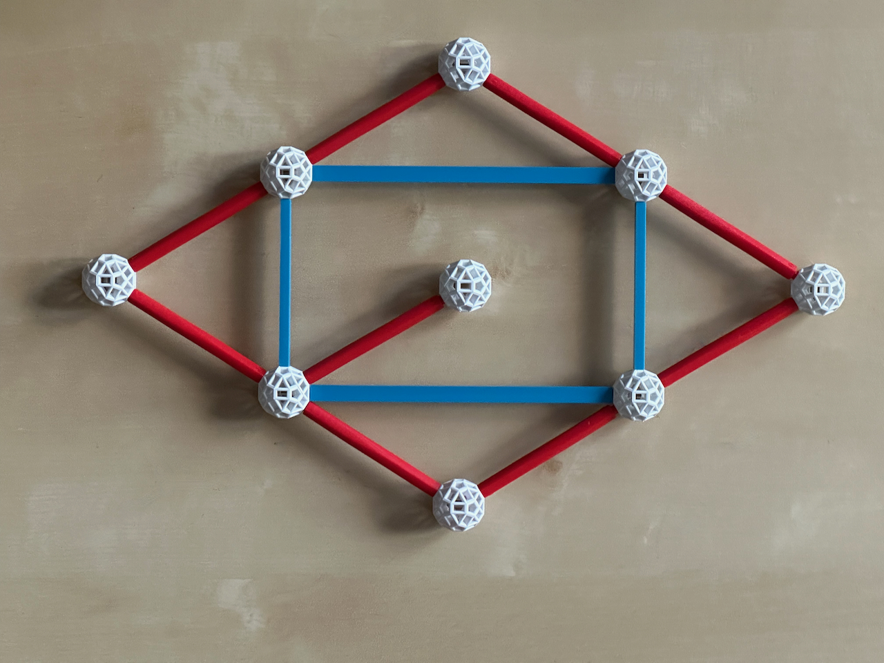
Fig. 2.5b: The rectification of a Golden rhombus is a Golden rectangle.
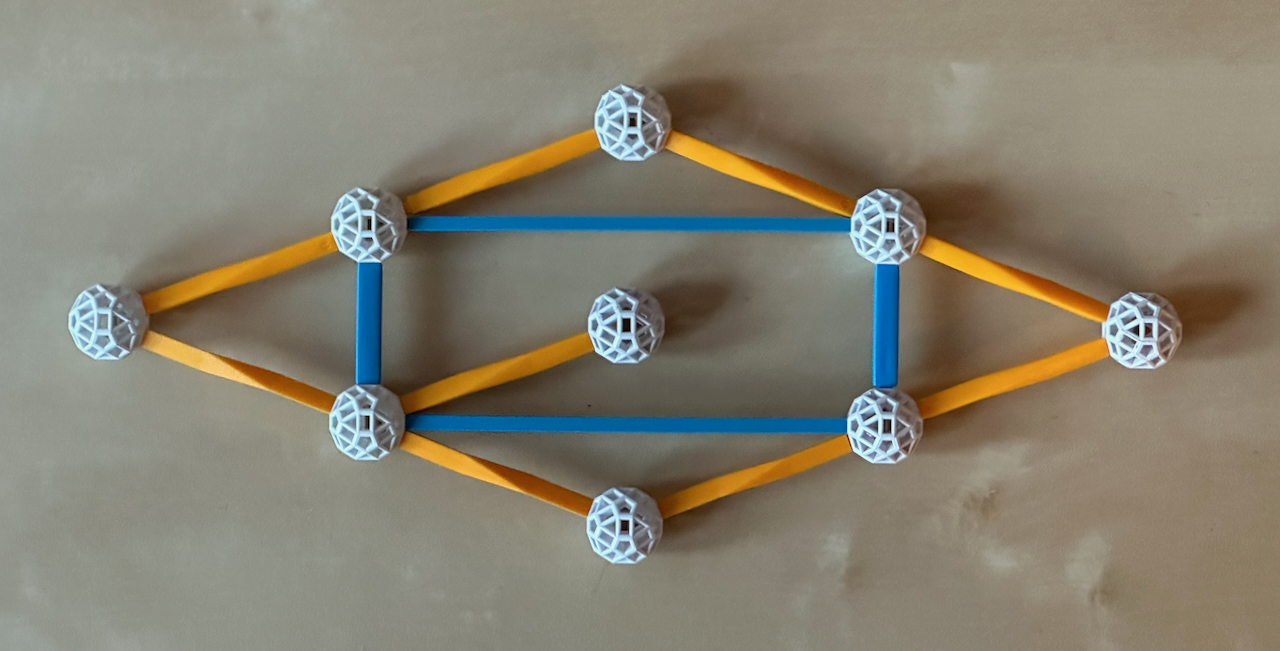
Fig. 2.5c: The rectification of a Long yellow rhombus is a Long yellow rectangle.
Note that the sides of the rhombuses are as long as the diagonals of the rectangles. Also,
it should be clear that the rectifications of these Rectangles results again in the
original rhombuses, but with half the size.
The rectifications of Figs. 2.5a, b and c are special cases of rectifications of
quadrilaterals, which by Varignon's theorem are
always parallelograms.
Stellation and faceting: A stellation
extends the edges of a polygon until they meet other similarly extended edges of the same
polygon. Stellations can transform a Polygon into a larger star polygon. The simplest case
is that of the Pentagon (if we stellate Triangles and Squares, their edges would never
meet), which stellates into a Pentagram (see Figure).
Facetings cut into a polygon, but preserve its vertices. Like the stellations, they cannot
be convex. In Fig. 2.3e, we saw two examples of faceting: the two tripods are facetings of
the ditrigon. In what follows we show additional examples of facetings.
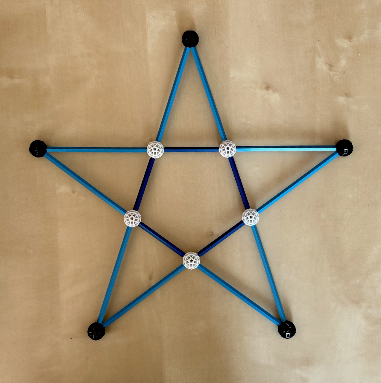
Fig. 2.6a: By extending the edges of the inner Pentagon, with vertices in white and dark
blue B1 struts, the stellation operation results in a Pentagram, with vertices in black.
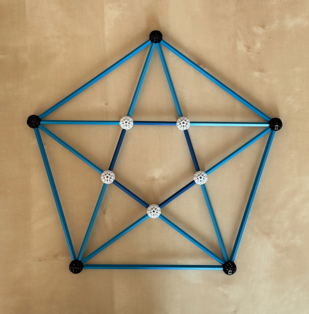
Fig. 2.6b: The Pentagram can be inscribed in a larger Pentagon, also with black vertices
and B3 struts, i.e., φ2 larger than the side of the inner Pentagon. In
this Figure, there are 15 Golden Gnomons and 20 Golden triangles.
In Fig. 2.6a, the inner white vertices are false vertices of the Pentagram. The new
Triangular areas that were added with the stellation of the Pentagon are Golden triangles;
with the two larger sides being equal to the diagonal of the Pentagon, φ times its
side (Figs. 2.1a, b). Thus, the side of the Pentagram is 1 + 2 φ = φ3
the side of the inner Pentagon.
In Fig. 2.6b, we inscribe the Pentagram in a larger Pentagon, which as can see, is the
dual of the inner Pentagon (see Fig. 2.4d). Because the real vertices are the same (in
black), the Pentagram is a faceting of the outer Pentagon. The sides of the Pentagram are
the full set of diagonals of the outer Pentagon. Since the diagonals are φ times
larger then the side of the outer Pentagon (see Figs. 2.1a, b), that side is only
φ2 larger than the side of the inner Pentagon. We see how these diagonals
divide the whole surface of the outer Pentagon into Golden triangles, gnomons and a
smaller Pentagon. This can be done again for the inner Pentagon, again and again ad
infinitum.
In the next figure, we stellate a Hexagon. This results is a regular compound of two
Triangles with sides three times larger, the Hexagram. This is the simplest of the
regular polygon compounds, the polygrams. This Hexagram can
be inscribed in a larger dual Hexagon, which it facets. As we've seen in Fig. 2.3e, there
are star hexagons, but none of them is regular.
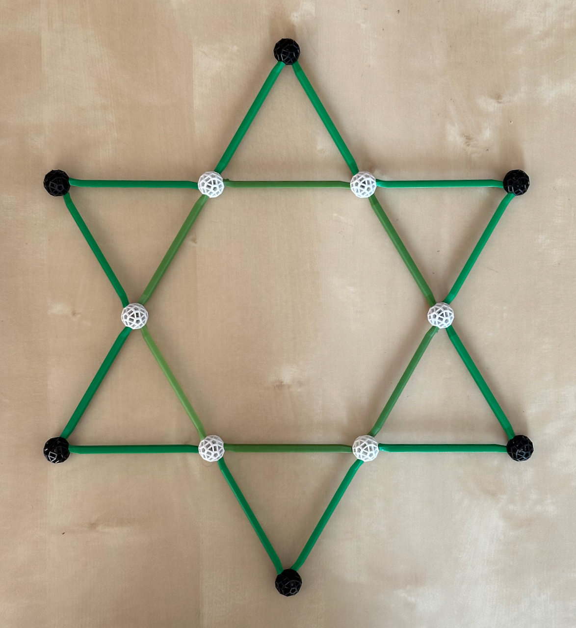
Fig. 2.7: The stellation transforms the inner Hexagon, with vertices in white and light
green G1 struts, into a regular polygon compound, the Hexagram, with vertices in black.
The inner white vertices are false vertices of the Hexagram.
The larger the number of sides/vertices of a polygon, the larger the number of distinct
stellations and facetings. This is, as we'll see now, the case of the Decagon, for which
we show all three distinct stellations. The first is a Polygram, consisting of two
Pentagons. The second is a regular star polygon, the Decagram. The third is
another Polygram, a compound of two Pentagrams. All of these are also facetings of of the
Decagon.
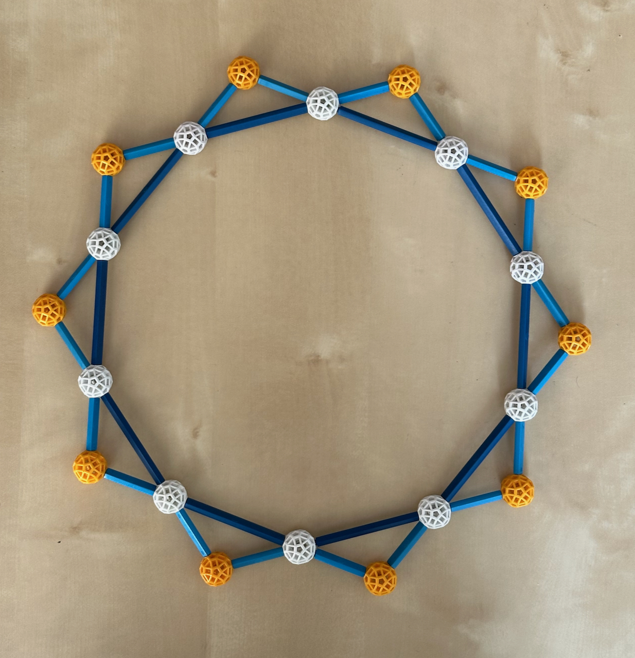
Fig. 2.8a: The first stellation of the Decagon (here in dark blue B1 struts and white
vertices) is a compound of two Pentagons, here with yellow vertices. The white vertices
further in are now false vertices.
2.8b: The second stellation of the Decagon is the Decagram, here with black vertices. The
white and yellow vertices further in are now false vertices.
Fig. 2.8c: The Decagram can be inscribed in a Decagon, which has edges built with B2
struts.
Notice how the radial struts bissect the quadrilaterals into Golden triangles, they also
define central Golden triangles. Notice too the three sizes of Golden gnomons.
Fig. 2.8d: The third and last stellation of the Decagon is a compound of two Pentagrams,
here with red vertices. These also result from stellating the two Pentagons with yellow
vertices. The white, yellow and black vertices further in are now false vertices. Figures
2.8c and d show how many times φ appears in these geometric objects.
In Fig. 2.8b, the side of the Decagram is represented by three B1 and two B0 struts, which
means it has a length 3 + 2 / φ = 1 + 2 φ = φ3 larger than the side
of the inner Decagon, represented by B1 struts. Importantly, this is the same proportion
as for the Pentagram and Pentagon.
In Fig. 2.8c, we inscribe this Decagram within a large Decagon. Since the real vertices
are the same (in black), this means that the Decagram is a faceting of the outer Decagon.
The latter is φ times larger but has, importantly, the same orientation of the inner
Decagon. The distance of a vertex to the center, which was φ, now becomes φ + 1 =
φ2.
Isomorphism: The Pentagon and Pentagram are isomorphic: they have same number of
sides and vertices with the same topology (a single circuit going
through five vertices and sides). They have the same configuration matrix. The same happens for
the Decagon and Decagram. However, the Hexagon and the Hexagram are not isomorphic, since
in the latter case there is not a single circuit that cover all vertices, but two (the two
Triangles of the compound) - the two figures have different topologies.
Metric properties and symmetry
In this page, I will not dwell much on the mathematical aspects of polytopes; the references cover that very well. However, a
few of the metric properties of polygons keep reappearing and being useful for
understanding the polytopes in this page. For this reason I will discuss them here. I will
however, make a couple general remarks about their symmetries first.
Some polygons have central symmetry: each element
is reflected through the centre of the polygon into an identical one. In such polygons not
only must the number of sides / vertices be even (as for instance, in the aforementioned
rectangles and rhombuses), but also the symmetry of the figure must be even. As an
example, the ditrigons and tripods in Fig. 2.3e (and their duals, the triambuses) have an
even number of sides (6), but because their overall symmetry is Triangular (order 3), they
have no central symmetry. This will be important for understanding rectified and partially
regular polytopes.
The regular polygons are much more symmetric, having dihedral symmetry. If their number
of sides / vertices is even, then they automatically have central symmetry, which is in
that case a sub-symmetry within the dihedral symmetry. Thus, if a Polygon has central
symmetry, its number of vertices/sides must be even.
The idea of a polygon as a circuit mentioned above will be discussed in more detail now.
As we go around a polygon, we pass through n vertices, while completing p turns around the
centre. For convex Polygons, p =1, but for the Pentagram, we actually complete two turns
around the centre, and for a Decagram 3 turns. This number is known as the polygon's
density.
If there are common factors in n and p, we are in the presence of a Polygram. For
instance, in Fig. 2.7, n = 6 and p = 2, hence two is a common factor, and thus we have 2
independent circuits (Polygons), each with n / p = 3 sides. Equally, for Fig. 2.8a, n = 10
and p = 2; 2 is the common factor and because of this we have 2 Polygons, each with n / p
= 5 sides. Finally, in Fig. 2.8d, n = 10 and p = 4, 2 is a common factor, so we have 2
Polygons, each with n = 5 and p = 2, i.e., two Pentagrams.
The angle subtended by two vertices as seen from the centre must add to 360 degrees
× p:
α = 360 p / n,
This angle is also the change of direction at each vertex, as we move from one side to the
next. Thus, the inner angle at the vertex is the supplementary angle:
β = 180 − 360 p/n.
These angles are listed in Table 1 below, for instance, for a Triangle, the inner angles
are 60 degrees. The sum is therefore 180 degrees. This sum is valid for all triangles in
flat, Euclidean spaces. For the Pentagon, we obtain the aforementioned inner angle of 108
degrees.
Fig. 2.9: Definition of the main angles of a Polygon. The black circle circunscribes the
Polygon, and has radius R0, the side is given by ℓ.
Now, if the vertices are at distance R0 from the centre (see Fig. 2.9), the
sides (with length ℓ) are the chord of
α times R0:
ℓ = R0 chord(α)
Replacing the sine expression of the chord and solving for R0, we obtain (see
also Fig. 2.9):
R0 = ℓ / (2 sin (α / 2)) = ℓ / ( 2 sin (180 p / n))
The minimum distance of the side to the centre is given by:
R1 = √ (R02 − (ℓ / 2)2) = ℓ / (2 tan (α / 2)) = ℓ / (2 tan (180 p / n))
The surface of the Polygon is the same as that of 2 n triangles with base ℓ/2 and
height R1.
Another important quantity is chord(β). This is, for any particular vertex P, the
distance between the two vertices it connects to divided by their distance from P (ℓ).
In Fig. 2.1a, the diagonal of the Pentagon has length L = chord(β) ℓ;
L is the side of the inscribed Pentagram (Fig. 2.6b). Generally chord(β) ℓ
is the side of the first faceting of a convex Polygon of side ℓ.
A consequence of the Zomable Polygons being constructible is that the sines in the
equations for R0, R1 and chord(β) are a subset of the
constructible numbers, the exact trigonometric
values. From these, we obtain the values listed below:
|
| Polygon |
α |
β |
R0/ℓ |
R1/ℓ |
chord(β) |
|
| Triangle | 120 | 60 | 1 / √3 | 1 / (2 √3) | 1 |
| Square | 90 | 90 | √2 / 2 | 1 / 2 | √2 |
| Hexagon | 60 | 120 | 1 | √3 / 2 | √3 |
|
| Pentagon | 72 | 108 | √( (5 + √5) / 10) | 1 / (2 √(5 − 2 √5)) | (√5 + 1) / 2 |
| Decagon | 36 | 144 | (√5 + 1) / 2 | √(5 + 2 √5) / 2 | √((5 + √5) / 2) |
| Pentagram | 144 | 36 | √2 / √(5 + √5) | 1 / (2 √(5 + 2 √5) ) | (√5 − 1) / 2 |
| Decagram | 108 | 72 | (√5 − 1) / 2 | √5 / (2 √(5 + 2 √5)) | √2 √(5 − √5) / 2 |
|
Table 1: Metric properties of Zomable Polygons
Some R0 lengths and chords are indicated in boldface because they are Zomable:
- For the Square, the R0 = √2/2 ℓ can be represented by the HG1 and
B1 struts in Fig. 2.3b. For the Hexagon, the R0 = ℓ implies it is, as
mentioned above, radially equilateral, as represented by the B1 and G1 struts from the
vertex to the centre in Fig. 2.3c.
- For the Decagon and Decagram, R0 = φ ℓ and R0 = 1 /
φ ℓ respectively, as shown in Figs. 2.3d and 2.8c.
- For the Pentagon and Pentagram, chord(β) = φ and 1/φ respectively, as
shown in Figs. 2.1a and 2.6b.
Regarding the Decagram,
- In Fig. 2.8b it results from stellating the Decagon in Fig. 2.3d. If for the Decagon
ℓ = 1 (a B1 strut), then for the Decagram ℓ = 3 + 1/φ = 1 + 2φ =
φ3. Importantly, this is also the ratio between the side of the Pentagram
and the the side of the Pentagon it stellates!
- For the Decagon R0 = φ (seen in its decomposition into Golden triangles
in Fig. 2.3d), for the Decagram R0 = φ + 1 = φ2 (Fig.
2.8c); thus confirming the R0 = 1 / φ ℓ relation for the Decagram.
- The radial of the Decagram was not represented with a B3 strut because the vertices of
the Decagon are in the way, i.e., the vertices of the outer Decagram are ``above'' those
of the Decagon, not in dual positions. The vertex arrangement of the Decagram is φ
times larger that for the vertices of the Decagon is stellates (Fig. 2.8c).
These properties will be important for a few polytopes to be mentioned later!
Paulo's polytope site / Next: Polyhedra